Earthquakes in the Landscape of Neural Network
Introduction
Artificial neural networks have been proven to be a very powerful tool for solving a wide variety of problems. Large number of researchers and engineers put their time and effort to develop the field, although there is still a lot to discover. And because of that, field evolves so quickly that large number of architectures and techniques that were popular just a few years ago, now is a part of the history. But not everything gets outdated and certain techniques prove to be useful to such an extent that it’s hard to imagine deep learning without them.
In this article, I want to direct your attention to the less known properties of one, quite famous, technique in the deep learning. I want to show you how beautiful and interesting could be a concept that typically left behind because of all more exciting ideas in this area.
What can you see?
Until now, I haven’t explained this mysterious “earthquake” phenomena and I would like to keep it like this for a little longer. I want to encourage you to focus on the properties of this phenomena and see whether you can recognize something that, most likely, is known to you.
As I mentioned earlier, certain clues could be revealed from the animation. In order to simplify things, we can focus our attention on a single frame and see what we can find.
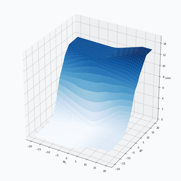
Some of you should be familiar with the graph like this. There we can see three axes, namely \(W_1\), \(W_2\) and Loss. Two of the axes specify different parameters/weights of the network, namely \(W_1\) and \(W_2\). The last axis shows a loss associated with each possible pair of parameters \(W_1\) and \(W_2\). That’s how neural network’s loss landscape looks like. Typically, during the training, we start with some fixed values \(W_1\), \(W_2\) and, with the help of an algorithm, like gradient descent, we navigate around landscape trying to find weights associated with lowest value on this surface. Assuming that this part is clear, one question still remains: Why does the loss landscape changes on the animation?
Let’s think what does this change represent. For each fixed pair of weights \(W_1\), \(W_2\) the loss value, associated with them, changes. And from this perspective it shouldn’t be that surprising, since we will never expect network to have exactly the same loss associated with a fixed set of weights. And at this point I would like to stop, since we’re getting pretty close to the answer.
I would encourage you to take a moment, think about what we’ve observed so far from the animation and guess what might produce this effect on the loss landscape. I suggest you to do it now, because next section contains an explanation of this phenomena.
Explanation
The animation shows how the neural network’s loss landscape looks like during the training with mini-batches. It’s quite common to think of a surface as a static landscape where we navigate during the training, trying to find weights that minimize desirable loss function. This statement might be considered as true only in case of the full-batch training, when all the available data samples are used at the same time during the training. But for most of the deep learning problems, that statement is false. During the training, we navigate in dynamically changing environment. For each training iteration, we take a set of input samples, propagate them thought the network and estimate gradient which we will use to adjust network’s weights.
It might be easier to visualize training using contour plots. The same 3D animation could be represented in the following way:
Animation above shows only the way the loss landscape changes when we use different mini-batches, but it doesn’t show us its effect on the training. We can extend this animation with gradient vectors.
Animation above alternates between two steps, namely training iteration and mini-batch changing. Training iteration shows static landscape and vector shows how the weights have changed after the update. Next training iteration requires different mini-batch and this changeover is visualized by the smooth transition between two landscapes. In reality, this change is not smooth, but animation helps us to notice the effect of that change. The bigger the difference between two losses the more noticeable will be transition between two landscapes.
After completing multiple training iterations, we can see that the overall path looks a bit noisy. During each iteration gradient point towards the direction that minimizes the loss but continuous changes in the loss landscape makes it quite difficult to find a stable direction. This problem could be minimized with algorithms that accumulate information about a gradient over time. If you want to learn more about that you can check this article.
Mathematical perspective
Unlike in mathematical optimization, in neural networks, we don’t know what function we want to optimize. It sounds a bit strange, but that’s true. Each mini-batch creates a different loss landscape and during each iteration we optimize different function. With random shuffling and reasonably large mini-batch size, it’s quite unlikely that we will see exactly the same loss landscape twice during the training. It sounds even a bit surreal, if you think about it. We move towards the minimum of the function which we most likely won’t see ever again and somehow optimization algorithm arrives at a solution that works incredibly well for a target task, e.g. image classification.
Most of the loss functions used in deep learning calculate loss independently per each input sample and the overall loss will be just an average of these losses. Notice, that this property helps us to obtain gradient very easily, since the gradient of the average is the average of the gradients per each individual addend.
where, N is the number of samples in a mini-batch, E is a total loss, \(e_i\) is a loss associated with i-th input sample.
We can think that during the training we randomly sample loss landscapes and use average loss landscape in order to estimate the gradient. For example, we can take 9 random input samples and create loss landscape per each individual sample. By averaging these landscapes, we can obtain new landscape.
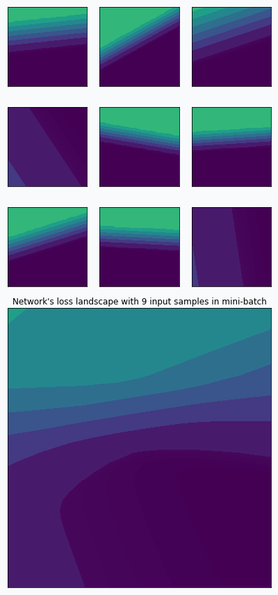
On the graph above, you can notice that 9 loss landscapes have linear contours and the averaged loss landscape doesn’t have this property. Each individual loss landscape has been obtained from a cross entropy loss function and simple logistic regression as a base network architecture. It could be easily shown that each individual loss is nearly piecewise linear function.
where \(x\) is an input vector, \(y \in \{0, 1\}\) is a target class and \(w\) is a vector with network’s parameters.
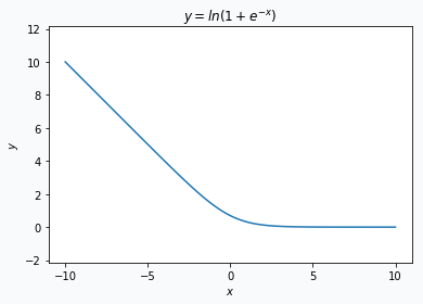
Obtained result could be separated into 2 parts. The first part is just a linear transformation of the input \(x\). The second part is a logarithm, but it behaves like a linear function when the absolute value of the \(x^T w\) is reasonably large.
Statistical perspective
We can also think about mini-batch training in terms of the loss landscape sampling. In statistics, random sampling helps us to derive properties of the entire population using summary statistics. For example, we might estimate expected value from the population by calculating average over a random sample. Obviously, the smaller sample we get, the less certain we’re about our estimation. And the same is true (or rather nearly true) for loss landscape sampling. This effect was demonstrated on the first animation:
I used mini-batch of size 10 for the graph on the left and size 100 for the graph on the right. We can see that “earthquake” effect is stronger for the left graph, where mini-batch size is smaller. Basically, estimation of the loss landscape, produced by small mini-batch, has quite large variance and it could be observed from the animation.
I want to make one disclaimer about sampling. It’s not quite the same as I’ve defined it for the statistical inference. Training dataset is already a sample from a population and each mini-batch is a sample from this sample. In addition to that, each mini-batch is not sampled independently. Typically, before each training epoch, we shuffle samples in our dataset and divide them into mini-batches. Propagation of the first mini-batch has an impact on the data distribution in the next mini-batch. For example, imagine simple problem where we try to classify 0 and 1 digits (binary classification on binary digits). In addition, we can imagine that in our training dataset, there are as many 0s as 1s. Imagine that in the first mini-batch we have more 1s than 0s. It means that in the rest of the training dataset we have more 0s than 1s and for the next mini-batch, we’re more likely to get more 0s than 1s, since probability was skewed by the first mini-batch. Whether it’s good, bad or shouldn’t matter, might be a separate topic for a different article, but the fact is that this sampling is not purely random.
Final words
In my opinion, term earthquake fits very naturally into a general intuition about neural network training. If you think about loss landscape as an area with mountains and valleys then earthquake represents shakes and displacement of that land. Magnitude of that earthquake could be measured with a size of the mini-batch. And navigation in this environment could be compared to the training with momentum.
Code
All the code, that has been used to generate graphs and animations for this article, could be found on Github.
Making Art with Growing Neural Gas
Introduction
I’ve been trying to make that type of art style for quite some time. I applied SOFM to the images, but in most cases it was unsuccessful, mostly because SOFM requires predefined size and structure of the network. With such a requirement it’s difficult to construct tool that converts image to nice art style. Later, I’ve learned more about Growing Neural Gas and it helped to resolve main issues with SOFM. In this article, I want to explain how this type of art style can be generated from the image. At the end, I will cover some of the similar, but less successful application with growing neural gas for image processing that I’ve been trying to develop.
Image Processing Pipeline
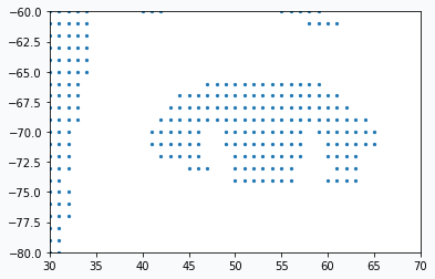
Images are not very natural data structure for most of the machine learning algorithms and Growing Neural Gas (GNG) is not an exception. For this reason, we need to represent input image in format that will be understandable for the network. The right format for the GNG would be set of data points. In addition, these data points have to somehow resemble original image. In order to do it, we can binarize our image and after that, every pixel on the image will be either black or white. Each black pixel we can use as a data point and pixel’s position as a feature. In this way, we would be able to extract topological structure of the image and store it as set of data points.
Conversion from the color image to binary image requires three simple image processing steps that we will apply in sequential way.
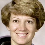
We need to load our image first
# skimage version 0.13.1
from skimage import data, img_as_float

astro = img_as_float(data.astronaut())
astro = astro[30:180, 150:300]
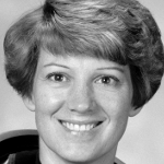
Convert color image to grayscale
from skimage import color
astro_grey = color.rgb2grey(astro)
Apply gaussian blurring. It will allow us to reduce image detalization.
from skimage.filters import gaussian
blured_astro_grey = gaussian(astro_grey, sigma=0.6)

Find binarization threshold and convert to the black color every pixel that below this threshold.
from skimage.filters import threshold_otsu
# Increase threshold in order to add more
# details to the binarized image
thresh = threshold_otsu(astro_grey) + 0.1
binary_astro = astro_grey < thresh
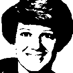
In some cases, it might be important to adjust threshold in order to be able to capture all important details. In this example, I added 0.1 to the threshold.
And finally, from the binary image it’s easy to make data points.
data = []
for (x, y), value in np.ndenumerate(binary_astro):
    if value == 1:
        data.append([y, -x])

plt.scatter(*np.array(data).T)
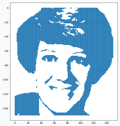
In the image there are so many data points that it’s not clear if it’s really just a set of data points. But if you zoom in you will see that they really are.
We prepared our data and now we need to learn a bit more about GNG network.
Growing Neural Gas
Growing Neural Gas is very simple algorithm and it’s really easy to visualize it. From the animation above you can see how it learns shape of the data. Network, typically, starts with two random points and expands over the space.
In the original paper [1], algorithm looks a bit complicated with all variables and terminology, but in reality it’s quite simple. Simplified version of the algorithm might look like this:
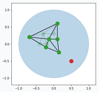
Pick one data point at random (red data point).
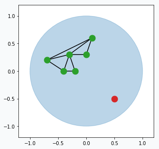
Blue region represents large set of data points that occupy space in the form of a unit circle. And green points connected with black lines is our GNG network. Green points are neurons and black line visualize connection between two neurons.
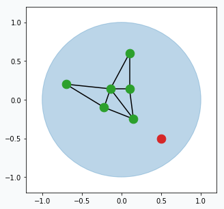
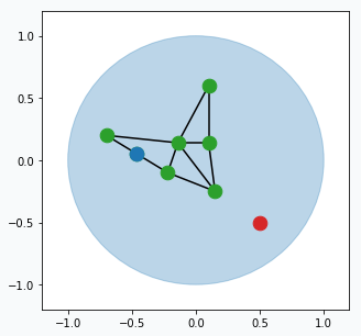
Find two closest neurons (blue data points) to the sampled data point and connect these neurons with an edge.
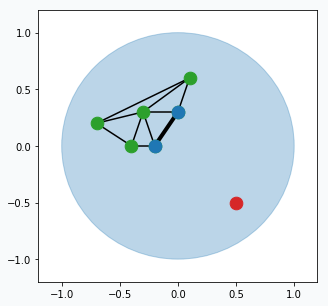
Move closest neuron towards the data point. In addition, you can move neurons, that connected by the edge with closest neuron, towards the same point.
Each neuron has error that accumulates over time. For every updated neuron we have to increase error. Increase per each neuron equal to the distance (euclidean) from this neuron to the sampled data point. The further the neuron from the data point the larger the error.
Remove edges that haven’t been updated for a while (maybe after 50, 100 or 200 iterations, up to you). In case if there are any neurons that doesn’t have edges then we can remove them too.
From time to time (maybe every 100 or 200 iterations) we can find neuron that has largest accumulated error. For this neuron we can find it’s neighbour with the highest accumulated error. In the middle way between them we can create new neuron (blue data point) that will be automatically connected to these two neurons and original edge between them will be destroyed.
You can think about this step in the following way. Find neuron that typically makes most errors and add one more neuron near it. This new neuron will help the other neuron to reduce accumulated error. Reduction in error will mean that we better capture structure of our data.
Repeat all the steps many times.
There are a few small extensions to the algorithm has to be added in order to be able to call it Growing Neural Gas, but the most important principles are there.
Putting Everything Together
And now we ready to combine power of the image processing pipeline with Growing Neural Gas.
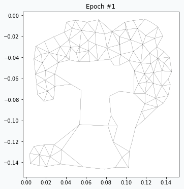
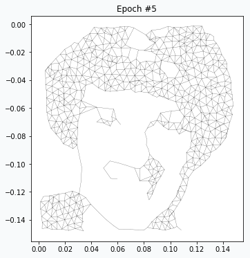
After running for one epoch we can already see some progress. Generated network resembles some distinctive features of our original image. At this point it’s pretty obvious that we don’t have enough neurons in the network in order to capture more details.
After 4 more iterations, image looks much closer to the original. You can notice that regions with large amount of data points have been developed properly, but small features like eyes, nose and mouth hasn’t been formed yet. We just have to wait more.
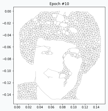
After 5 more iterations the eyebrows and eyes have better quality. Even hair has more complex shape.
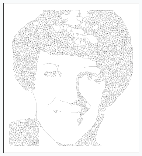
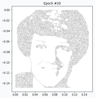
On the 20th iteration network’s training has been stopped since we achieved desired quality of the image.
Reveal Issues with More Examples
I’ve been doing some experiments with other image as well, and there are a few problems that I’ve encountered.
There are two main components in the art style generation procedure, namely: image processing pipeline and GNG. Let’s look at problem with GNG network. It can be illustrated with the following image.

If you compare horses you will notice that horse on the right image looks a bit skinnier than the left one. It happened, because neurons in the GNG network are not able to rich edges of the image. After one training pass over the full dataset each neuron is getting pulled from many directions and over the training process it settles somewhere in the middle, in order to be as close as possible to every sample that pulls it. The more neurons you add to the network the closer it will get to the edge.
Another problem related to the image binarization, the most difficult step in our image processing pipeline. It’s difficult, because each binarization method holds certain set of assumption that can easily fail for different images and there is no general way to do it. You don’t have such a difficulty with the network. It can give you pretty decent results for different images using the same configurations. The only thing that you typically need to control is the maximum number of neurons in the network. The more neuron you allow network to use the better quality of the image it produces.
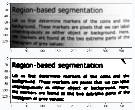
In this article, I used global binarization method for image processing. This type of binarization generates single threshold for all pixels in the image, which can cause problems. Let’s look at the image below.
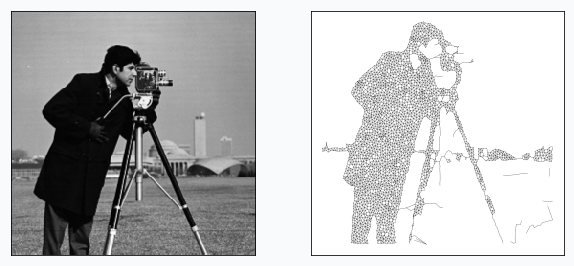
You can see that that there are some building in the background in the left image, but there is none in the right one. It’s hard to capture multiple object using single threshold, especially when they have different shades. For more complex cases you might try to use local thresholding methods.
Applying Similar Approach to Text
I’ve been also experimenting with text images. In the image below you can see the result.
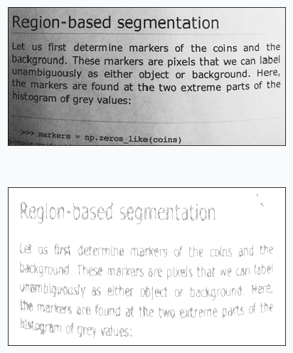
It’s even possible to read text generated by the network. It’s also interesting that with slight modification to the algorithm you can count number of words in the image. We just need to add more blurring and after the training - count number of subgraphs in the network.
After many reruns I typically get number that very close to the right answer (44 words if you count “Region-based” as two words).
I also tried to train GNG network that captures trajectory of the signature. There are a few issues that I couldn’t overcome. In the image below you can clearly see some of these issues.
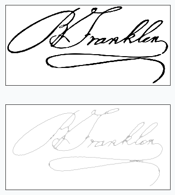
You will expect to see a signature as a continuous line and this property is hard to achieve using GNG. In the image above you can see a few places where network tries to cover some regions with small polygons and lines which looks very unnatural.
Final Words
Beautiful patterns generated from the images, probably, doesn’t reflect the real power of GNG network, but I think that the beauty behind algorithm shouldn’t be underappreciated only because it’s not useful for solving real world problems. There are not many machine learning algorithms that can be used for artistic application and it’s pretty cool when they work even though they weren’t designed for this purpose.
I had a lot of fun trying different ideas and I encourage you to try it as well. If you’re new to machine learning - it’s easy to start with GNG and if you’re an expert, I might try motivating you saying that it’s quite refreshing to work with neural networks that can be easily interpreted and analyzed.
Learn More
In case if you want to learn more about algorithms just like GNG then you can read about SOFM. As I said in the beginning of the article, it doesn’t work as nice as GNG for images, but you can write pretty cool text styles or generate beautiful patterns. And, it has some other interesting applications (even in deep learning).
Code
A few notebooks with code are available on github.
- Main notebook that generates all the images using GNG
- Growing Neural Gas animation notebook
- Notebook that generates step by step visualization images for the Growing Neural Gas algorithm
References
| [1] | A Growing Neural Gas Network Learns Topologies, Bernd Fritzke et al. https://papers.nips.cc/paper/893-a-growing-neural-gas-network-learns-topologies.pdf |
| [2] | Thresholding, tutorial from scikit-image library http://scikit-image.org/docs/dev/auto_examples/xx_applications/plot_thresholding.html |
| [3] | Thresholding (image processing), wikipedia article https://en.wikipedia.org/wiki/Thresholding_%28image_processing%29 |
Create unique text-style with SOFM
Introduction
In this article, I want to show how to generate unique text style using Self-Organizing Feature Maps (SOFM). I won’t explain how SOFM works in this article, but if you want to learn more about algorithm you can check these articles.
Transforming text into the data
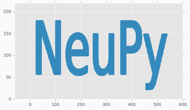
In order to start, we need to have some text prepared. I generated image using matplotlib, but anything else that able to generate image from the text will work.
import matplotlib.pyplot as plt

red, blue, white = ('#E24A33', '#348ABD', '#FFFFFF')

ax = plt.gca()
ax.patch.set_facecolor(white)
ax.text(0, 0.25, 'NeuPy', fontsize=120)

plt.xticks([])
plt.yticks([])

plt.savefig('neupy-text.png', facecolor=white, bbox_inches='tight')
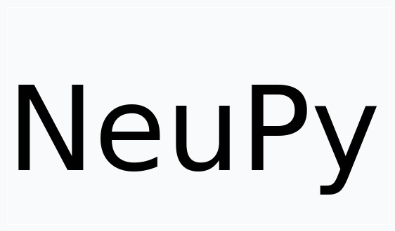
We cannot train SOFM using image, for this reason we will have to transform image into a set of data points. In order to do it we will encode every black pixel as data point and we will ignore white pixels. It’s hard to see from the picture, but not all pixels are black and white. If you zoom close enough you will see that there are some gray pixels near the edge of each letter. For this reason, we have to binarize our image first.
from scipy.misc import imread

neupy_text = imread('neupy-text.png')
# Encode black pixels as 1 and white pixels as 0
neupy_text = (1 - neupy_text / 255.).round().max(axis=2)
After binarization we have to filter all pixels that have value 1 and use pixel coordinates as a data point coordinates.
data = []
for (x, y), value in np.ndenumerate(neupy_text):
    if value == 1:
        data.append([y, -x + 300])

data = np.array(data)
We can use scatter plot to show that collected data points still resemble the shape of the main text.
plt.scatter(*data.T, color=blue)
plt.show()
Weight initialization
Weight initialization is very important step. With default random initialization it can be difficult for the network to cover the text, since in many cases neurons will have to travel across all image in order to get closer to their neighbors. In order to avoid this issue we have to manually generate grid of neurons, so that it would be easier for the network to cover the text.
I tried many different patterns and most of them work, but one-dimensional or nearly one-dimensional grids produced best patterns. It’s mostly because patterns generated using two-dimensional grid look very similar to each other. With one-dimensional grid it’s like covering the same text with long string. Network will be forced to stretch and rollup in order to cover the text. I mentioned term nearly one-dimensional, because that’s the shape that I used at the end. Term “nearly” means that grid is two-dimensional, but because number of neurons along one dimension much larger than along the other we can think of it as almost one-dimensional. In the final solution I used grid with shape 2x1000.
# This parameter will be also used in the SOFM
n = 1000
# Generate weights and arange them along sine wave.
# Because sine way goes up and down the final pattern
# will look more interesting.
weight = np.zeros((2, n))
# Width of the weights were selected specifically for the NeuPy text
weight[0, :] = np.linspace(25, 500, n)
# Amplitute of the sine function also was selected in order
# to roughly match height of the text
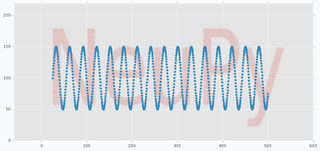
weight[1, :] = (np.sin(np.linspace(0, 100, n)) + 1) * 50 + 50
weight = np.concatenate([weight, weight], axis=1)
You can notice from the code that I applied sine function on the y-axis coordinates of the grid. With two-dimensional grid it’s easy to cover the text. We just put large rectangular grid over the text. With nearly one-dimensional grid it’s a bit tricky. We need to have a way that will allow us to cover our text and sine is one of the simple functions that can provide such a property. From the image below you can see how nicely it cover our text.
plt.figure(figsize=(16, 6))
plt.scatter(*weight, zorder=100, color=blue)
plt.scatter(*data.T, color=red, alpha=0.01)
plt.show()
Training network
And the last step is to train the network. It took me some time to find right parameters for the network. Typically it was easy to see that there is something wrong with a training when all neurons start forming strange shapes that look nothing like the text. The main problem I found a bit latter. Because we have roughly 20,000 data points and 2000 neurons we make to many updates during one iteration without reducing parameter values. Reducing step size helped to solve this issue, because every update makes small change to the grid and making lots of these small changes make noticeable difference.
from neupy import algorithms

sofm = algorithms.SOFM(
    n_inputs=2,
    features_grid=(2, n),
    weight=weight,

    # With large number of training samples it's safer
    # to use small step (learning rate)
    step=0.05,

    # Learning radis large for first 10 iterations, after that we
    # assume that neurons found good positions on the text and we just
    # need to move them a bit independentl in order to cover text better
    learning_radius=10,

    # after 10 iteration learning radius would be 0
    reduce_radius_after=1,

    # slowly decrease step size
    reduce_step_after=10,
)
Because of the small step size we have to do more training iterations. It takes more time to converge, but final results are more stable to some changes in the input data. It’s possible to speed up the overall process tuning parameter more carefully, but I decided that it’s good enough.
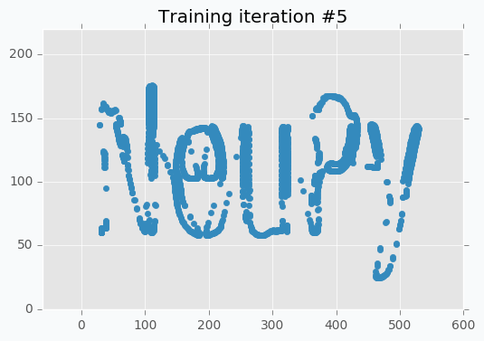
I run training procedure for 30 iterations.
for iteration in range(30):
    sofm.train(data, epochs=1)

    plt.title('Training iteration #{}'.format(iteration))
    plt.scatter(*sofm.weight, color=blue)
    plt.show()
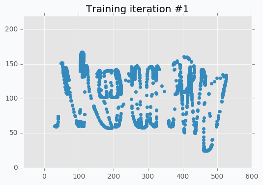
SOFM was trained for only one iteration and we already can vaguely see most of the latters. Let’s wait a few more iterations.
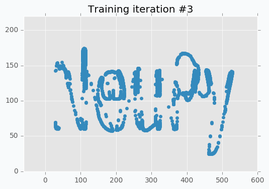
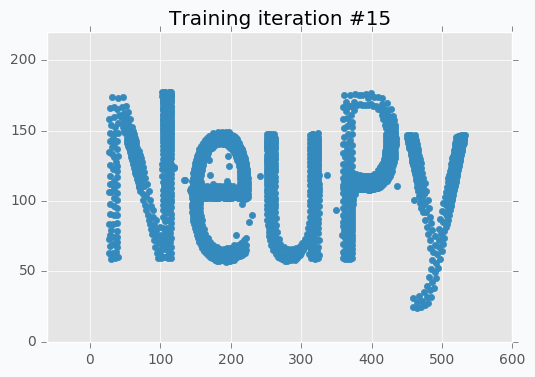
Now it’s way more clear that network makes progress during the training. And after 5 more iterations it’s almost perfectly covers text.

But even after 10 iterations we still can see that some of the letters still require some polishing. For instance, left part of the letter N hasn’t been properly covered.
In addition, it’s important to point out that we specified step reduction after every 10 iterations. It means that now we won’t move neurons as much as we did before. Also, learning radius was reduced to zero, which means that after 10th iteration each neuron will move independently. And these two changes are exactly what we need. We can see from the picture that network covers text pretty good, but small changes will make it look even better.
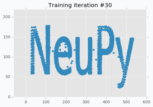
You can notice that there is almost no difference between iteration #15 and #30. It doesn’t look like we made any progress after 15th iteration, but it’s not true. If you stop training after 15th iteration, you will notice that some parts of the letters look a bit odd. These 15 last iterations do small changes that won’t be noticeable from the scatter plot, but they are important.
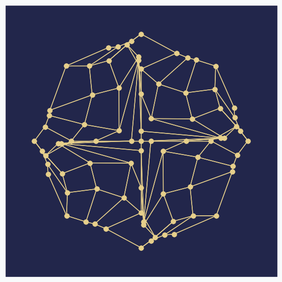
And finally after all training iterations we can use our weights to generate logo.
# Function comes from the neupy's examples folder
from examples.competitive.utils import plot_2d_grid

background_color = '#22264b'
text_color = '#e8edf3'

fig = plt.figure(figsize=(14, 6))
ax = plt.gca()
ax.patch.set_facecolor(background_color)

sofm_weights = sofm.weight.T.reshape((2, n, 2))
plot_2d_grid(np.transpose(sofm_weights, (2, 0, 1)), color=text_color)

plt.xticks([])
plt.yticks([])

# Coordinates were picked so that text
# will be in the center of the image
plt.ylim(0, 220)
plt.xlim(-10, 560)

plt.show()
Generalized approach for any text
There are some challenges that you can face when you try to adopt this solution for different text. First of all, from the code you could have noticed that I “hard-coded” bounds of the text. In more general solution they can be identified from the image, but it will make solution more complex. For instance, the right bound of the text can be associated with data point that has largest x-coordinate. And the same can be done for the upper bound of the text. Second problem is related to the parameters of the SOFM. The main idea was to make lots of small updates for a long time, but it might fail for some other text that has more letters, because we will have more data points and more updates during each iterations. Problem can be solved if step size will be reduced.
Further reading
If you want to learn more about SOFM, you can read the “Self-Organizing Maps and Applications” article that covers basic ideas behind SOFM and some of the problems that can be solved with this algorithm.
Code
All the code that was used to generate images in the article you can find in iPython notebook on github.
The Art of SOFM
Introduction
In this article, I just want to show how beautiful sometimes can be a neural network. I think, it’s quite rare that algorithm can not only extract knowledge from the data, but also produce something beautiful using exactly the same set of training rules without any modifications.
The main idea
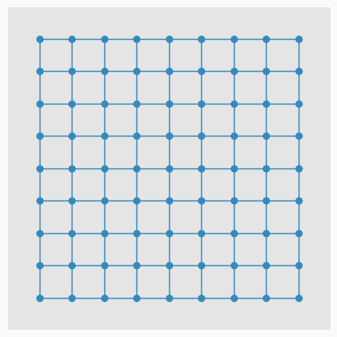
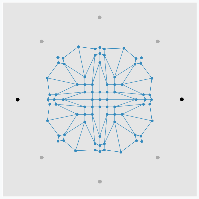
SOFM consists of multiple neurons that typically arranged in the grid with connections between some of the neurons. In this article, we will use grid in the shape of the square that looks like this.
During the training iteration we introduce some data point near the grid.
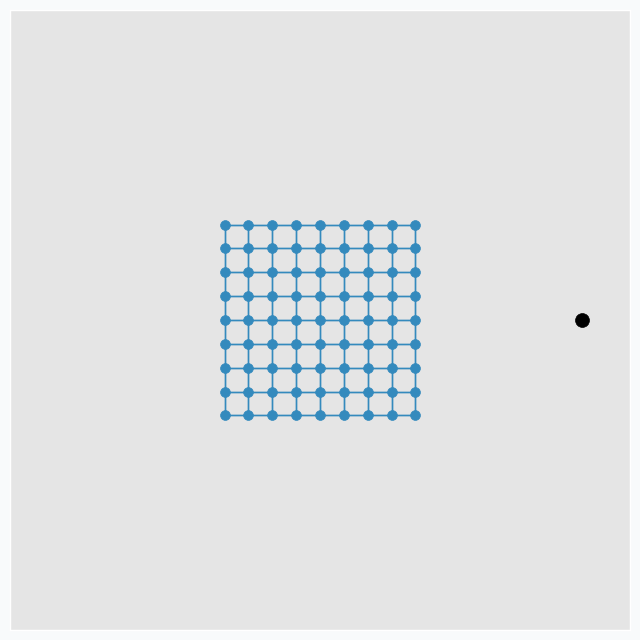
SOFM finds neuron that closest to the introduced data point. After that, it pushes neuron towards this data point. In addition, it finds a few neighbour neurons within specified radius, that we call learning radius, and pushes these neurons towards data point as well, but not as much as it pushed closest neuron.
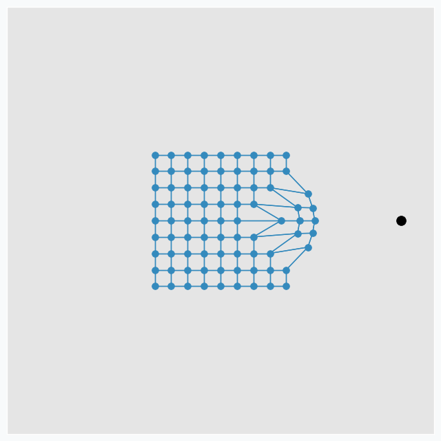
To make it more interesting, we can put few extra points around the same grid.
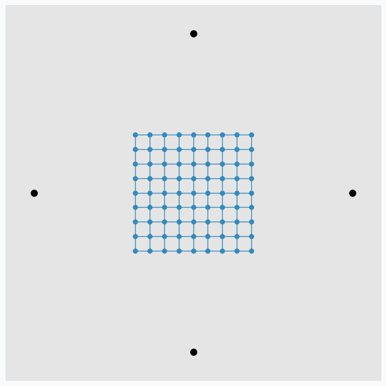
And applying one update per each data point at a time we can get nice pattern.
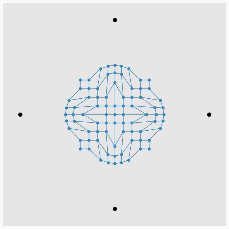
We can make patterns look more interestingly if we start moving data points around. Let’s now use only two points and put one on the left and one on the right side from the grid. We do the same SOFM update again, but as soon as it’s done we rotate two data points by 45 degrees counterclockwise. After repeating this process a few times, we can get another pattern.
Black dots are two initial data points. And gray dots show places where we’ve seen these two data points after each new 45 degree rotation.
It’s pretty cool that this simple approach can produce such a beautiful patterns. We can even define set of variables changing which we can generate different patterns.
Making patterns more interesting
Randomizing some of the SOFM parameters we can produce different patterns on each run. In this article, we will use 3 most important SOFM parameters:
- Learning rate
- Learning radius
- Learning rate for the neighbour neurons
Learning rate defines by how much we will push neurons during the updated. If learning rate value is small then we won’t push it to far from the initial position.
Learning radius defines how many neighbour neurons will be updated. The larger the radius the more neighbours would be updated after each iteration. If learning radius equal to zero then only one neuron will be updated.
And the last one is a parameter that controls learning rate for the neighbour neurons. The larger the value the bigger update neighbour neurons will get.
Generate interesting patterns
As in the example before, we will use only two data points and we will rotate them after each update by 45 degree counterclockwise. Each of the 3 SOFM parameter we randomly sample from the uniform distribution. Here are 16 randomly generated patterns.
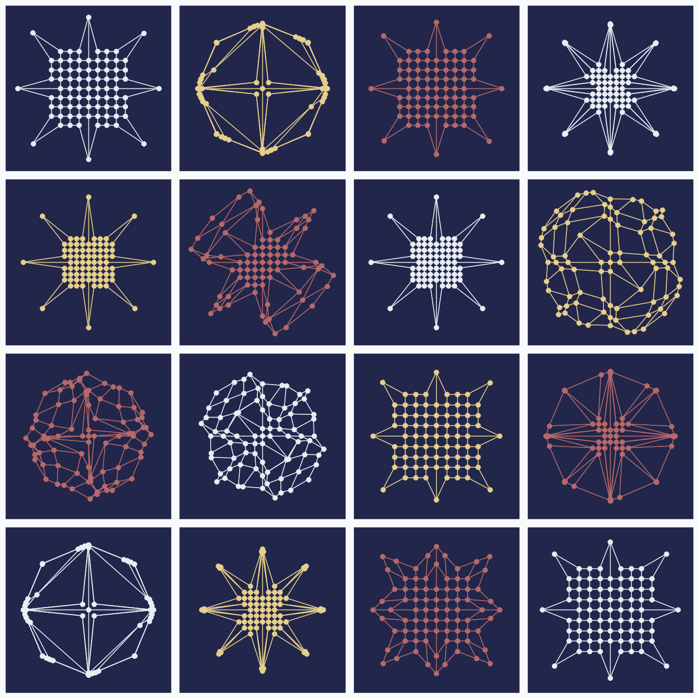
You can see that even small changes in some of the parameters can produce very different results. One of the patterns even look like a bird.
Applications
It looks a bit strange to think about this approach in context of practical applications, but there are some things that you can do with these patterns. For instance, it can be used to generate unique avatar images for the new website users. Adding more rules and variables to the image generating function we can make patterns even more diverse.
I also tried to play a game with these patterns in order to train my intuition. We use SOFM network parameters in order to generate these image, but reverse procedure is also possible. Seeing the generated pattern we can guess parameters that was used to generate it. For instance, here is a simple example of the pattern that looks like star
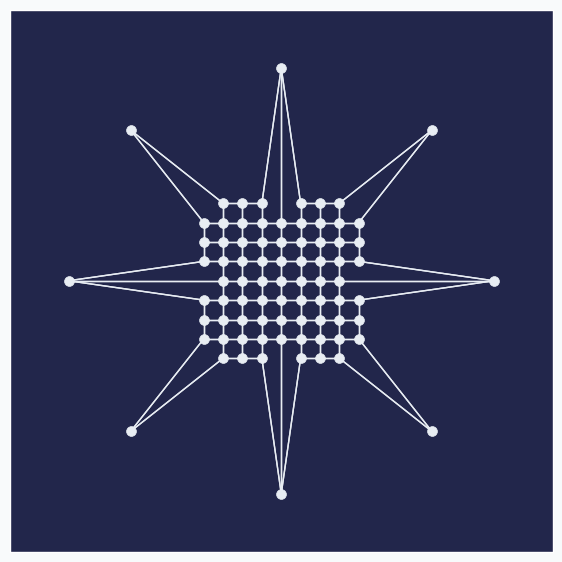
We can see that only one dot moved in each direction, so we can say that learning radius was zero. Since updated neurons moved far away from the initial grid we can say that learning rate was large.
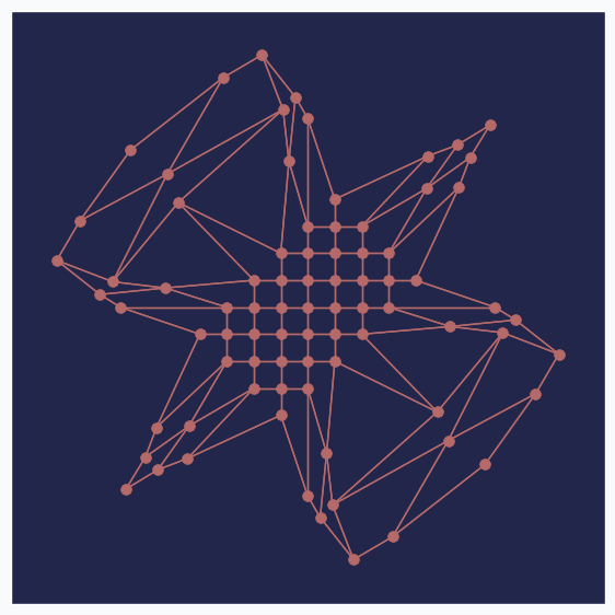
Here is another one, more complicated.
In this example it’s harder to say what happened, but we have at least one clue.In the center of the grid there are three dots, arranged horizontally, that didn’t move after all updates. Knowing that there are nine dots in the row, we can conclude that learning radius was 2 or 3. We not sure which one, but if you see that there are just 5 dots left on their initial positions then it’s very likely that radius was 3 since we moved more neurons into new positions.
I hope you got the idea. It’s not always possible to guess the exact values, but each pattern can reveal some clues about the algorithm’s set up.
Further reading
If you want to learn more about SOFM, you can check article that covers basic ideas behind SOFM and some of the problems that can be solved with this algorithm.
Code
All the code that was used to generate images in the article you can find in iPython notebook on github.
Self-Organizing Maps and Applications
Contents
Introduction
I was fascinated for a while with SOFM algorithm and that’s why I decided to write this article. The reason why I like it so much because it’s pretty simple and powerful approach that can be applied to solve different problems.
I believe that it’s important to understand the idea behind any algorithm even if you don’t know how to build it. For this reason, I won’t give detailed explanation on how to build your own SOFM network. Instead, I will focus on the intuition behind this algorithm and applications where you can use it. If you want to build it yourself I recommend you to read Neural Network Design book.
Intuition behind SOFM
As in case of any neural network algorithms the main building blocks for SOFM are neurons. Each neuron typically connected to some other neurons, but number of this connections is small. Each neuron connected just to a few other neurons that we call close neighbors. There are many ways to arrange these connections, but the most common one is to arrange them into two-dimensional grid.

Each blue dot in the image is neuron and line between two neurons means that they are connected. We call this arrangement of neurons grid.
Each neuron in the grid has two properties: position and connections to other neurons. We define connections before we start network training and position is the only thing that changes during the training. There are many ways to initialize position for the neurons, but the easiest one is just to do it randomly. After this initialization grid won’t look as nice as it looks on the image above, but with more training iteration problem can be solved.
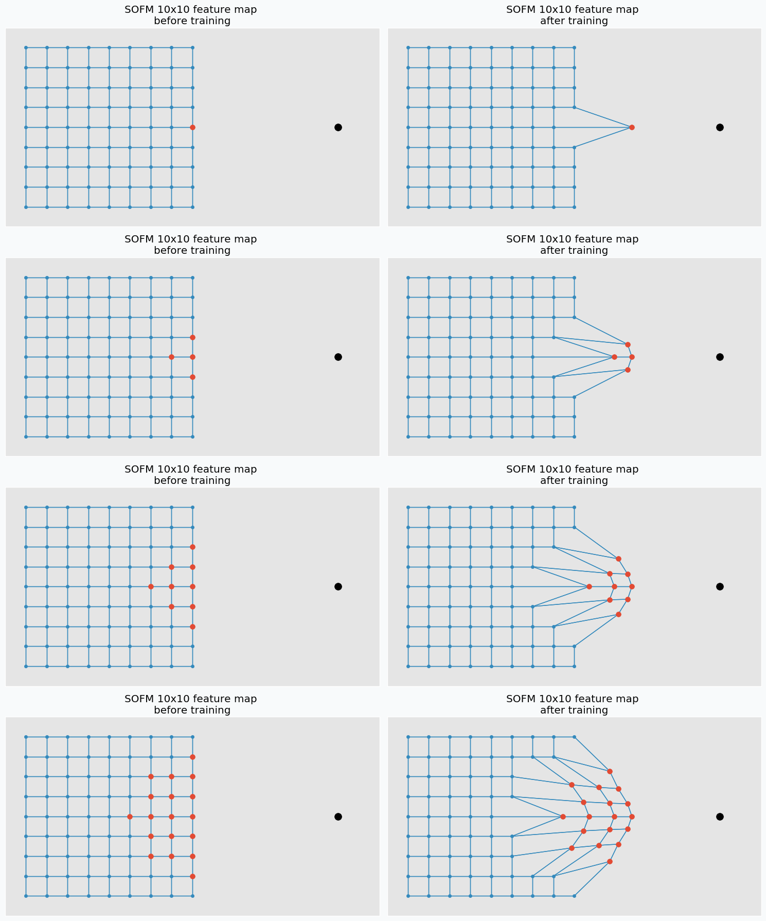
Let’s talk about training. In each training iteration we introduce some data point and we try to find neuron that closest to this point. Neuron that closest to this point we call neuron winner. But, instead of updating position of this neuron we find its neighbors. Note, that it’s not the same as closest neighbors. Before training we specify special parameter known as learning radius. It defines the radius within which we consider other neuron as a neighbors. On the image below you can see the same grid as before with neuron in center that we marked as a winner. You can see in the pictures that larger radius includes more neurons.
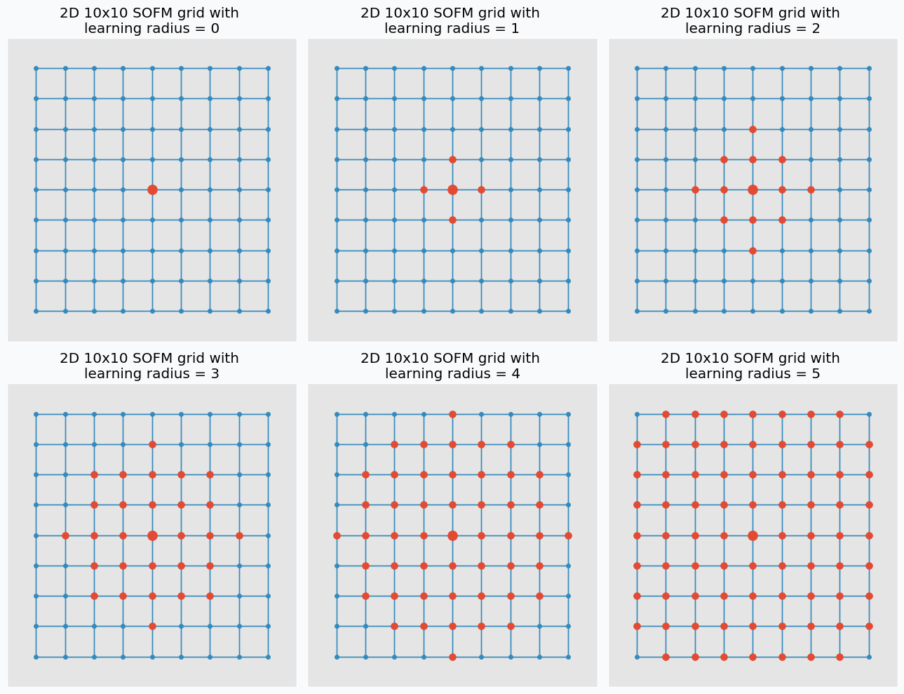
And at the end of the iteration we update our neuron winner and its neighbors positions. We change their position by pushing closer to the data point that we used to find neuron winner. We “push” winner neuron much closer to the data point compared to the neighbor neurons. In fact, the further the neighbors the less “push” it get’s towards the data point. You can see how we update neurons on the image below with different learning radius parameters.
You probably noticed that idea is very similar to k-means algorithm, but what makes it really special is the existing relations with other neurons.
It’s easy to compare this algorithm to real world. Imagine that you try to put large tablecloth on the large table. First you put it so that it will partially cover table. Then you will go around and pull different sides of the tablecloth until you cover the table. But when you pull one side, another part of the tablecloth starts moving to the direction in which you pull it, just like it happens during the training in SOFM.
Applications
Surprisingly, this simple idea has a variety of applications. In this part of the article, I’ll cover a few most common applications.
Clustering
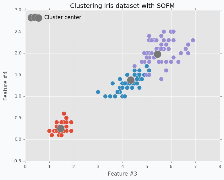
Clustering is probably the most trivial application where you can use SOFM. In case of clustering, we treat every neuron as a centre of separate cluster. One of the problems is that during the training procedure when we pull one neuron closer to one of the cluster we will be forced to pull its neighbors as well. In order to avoid this issue, we need to break relations between neighbors, so that any update will not have influence on other neurons. If we set up this value as 0 it will mean that neuron winner doesn’t have any relations with other neurons which is exactly what we need for clustering.
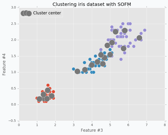
In the image below you can see visualized two features from the iris dataset and there are three SOFM neurons colored in grey. As you can see it managed to find pretty good centers of the clusters.
$ python sofm_iris_clustering.py
Clustering application is the useful one, but it’s not very special one. If you try to run k-mean algorithm on the same dataset that I used in this example you should be able to get roughly the same result. I don’t see any advantages for SOFM with learning radius equal to 0 against k-means. I like to think about SOFM clustering application more like a debugging. When you are trying to find where your code breaks you can disable some parts of it and try to see if the specific function breaks. With SOFM we are disabling some parts in order to see how other things will behave without it.
What would happen if we increase number of clusters? Let’s increase number of clusters from 3 to 20 and run clustering on the same data.
Neurons just spread out all over the data trying to cover it. Just in this case, since we have lots of clusters each one will cover smaller portion of the data. We can call it a micro-clustering.
Space approximation
In the previous example, we tried to do a space approximation. Space approximation is similar to clustering, but the goal is here to find the minimum number of points that cover as much data as possible. Since it’s similar to clustering we can use SOFM here as well. But as we saw in the previous example data points wasn’t using space efficiently and some points were very close to each other and some are further. Now the problem is that clusters don’t know about existence of other clusters and they behave independently. To have more cooperative behavior between clusters we can enable learning radius in SOFM. Let’s try different example. I generated two-dimensional dataset in the shape of the moon that we will try to approximate using SOFM. First, let’s try to do it without increasing learning radius and applying the same micro-clustering technique as before.
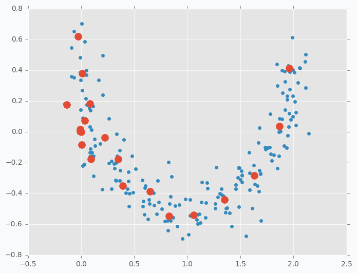
As you can see we have the same issue as we had with iris dataset. On the left side there are a few cluster centers that very close to each other and on the right side they are further apart. Now, let’s try to set up learning radius equal to 2 and let’s look what will happen.
$ python sofm_moon_topology.py
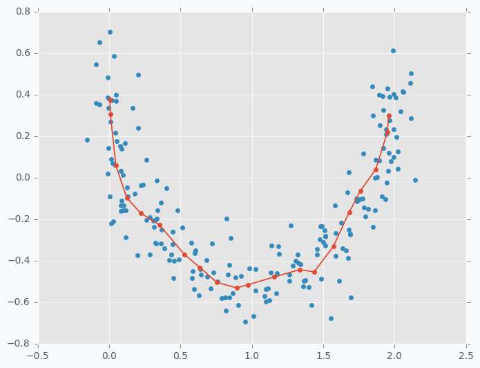
You can see that cluster centers are more efficiently distributed along the moon-shaped cluster. Even if we remove data points from the plot the center cluster will give us good understanding about the shape of our original data.
You might ask, what is the use of this application? One of the things that you can do is to use this approach in order to minimize the size of your data sample. The idea is that since feature map spreads out all over the space you can generate smaller dataset that will keep useful properties of the main one. It can be not only useful for training sample minimization, but also for other applications. For instance, in case if you have lots of unlabelled data and labelling can get expensive, you can use the same technique to find smaller sub-sample of the main dataset and label only this subset instead of the random sample.
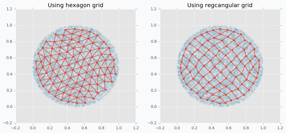
We can use more than one-dimensional grids in SOFM in order to be able to capture more complicated patterns. In the following example, you can see SOFM with two-dimensional feature map that approximates roughly 8,000 data points using only 100 features.
$ python sofm_compare_grid_types.py
The same property of space approximation can be extended to the high-dimensional datasets and used for visualizations.
High-dimensional data visualization
We used SOFM with two-dimensional feature map in order to catch dimensional properties of the datasets with only two features. If we increase number of dimensions to three it still would be possible to visualize the result, but in four dimensions it will become a bit trickier.
If we use two-dimensional grid and train SOFM over the high-dimensional data then we can encode network as a heat map where each neuron in the network will be represented by the average distance to its neighbors.
As the example, let’s take a look at the breast cancer dataset available in the scikit-learn library. This dataset has 30 features and two classes.
Let’s look what we can get if we apply described method on the 30-dimensional data.
$ python sofm_heatmap_visualization.py
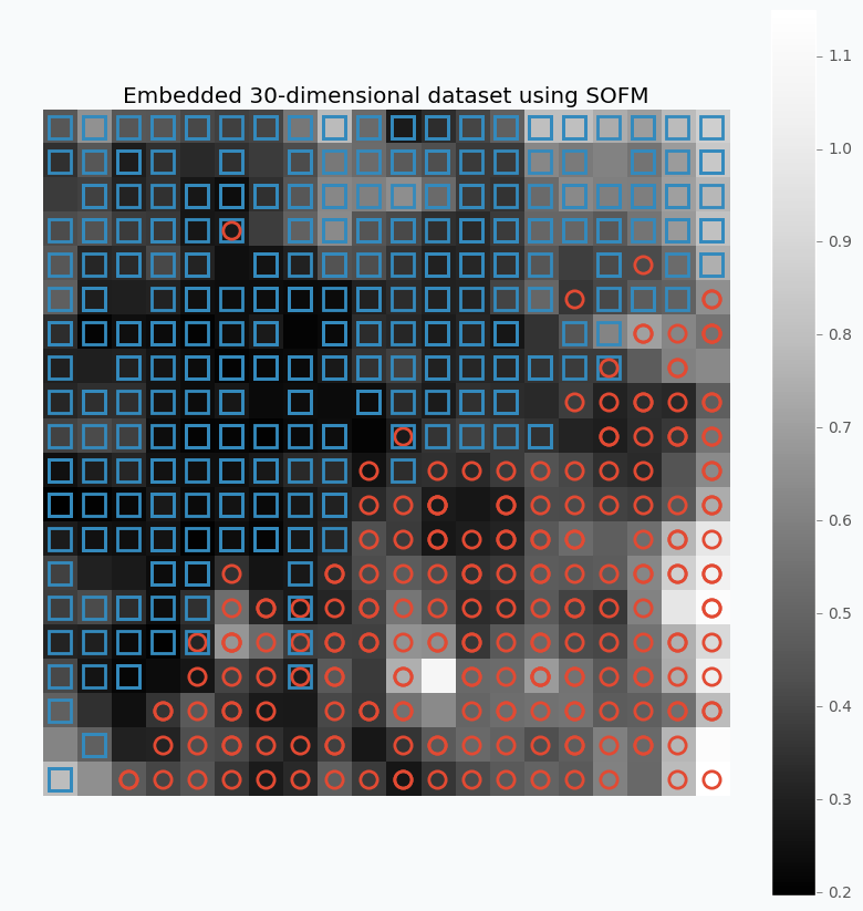
For this example, I used SOFM with 20x20 feature map. Which basically means that we have 400 micro-clusters. Most of the micro-clusters has either blue squares or red circles and just a few of them has both or none of the classes.
You can see how micro-clusters with blue squares are tended to be close to each other, and the same true for red circles. In fact, we can even draw simple bound that will separate two different classes from each other. Along this bound we can see some cases where micro-cluster has red and blue classes which means that at some places these samples sit very tight. In other cases, like in the left down corner, we can see parts that do not belong to any of the classes which means that there is a gap between data points.
You can also notice that each cell in the heat map has different color. From the colorbar, we can see that black color encodes small numbers and white color encodes large numbers. Each cell has a number associated with it that defines average distance to neighbor clusters. The white color means that cluster is far away from it’s neighbors. Group of the red circles on the right side of the plot has white color, which means that this group is far from the main cluster.
One problem is that color depends on the average distance which can be misleading in some cases. We can build a bit different visualization that will encode distance between two separate micro-clusters as a single value.
$ python sofm_heatmap_visualization.py --expanded-heatmap
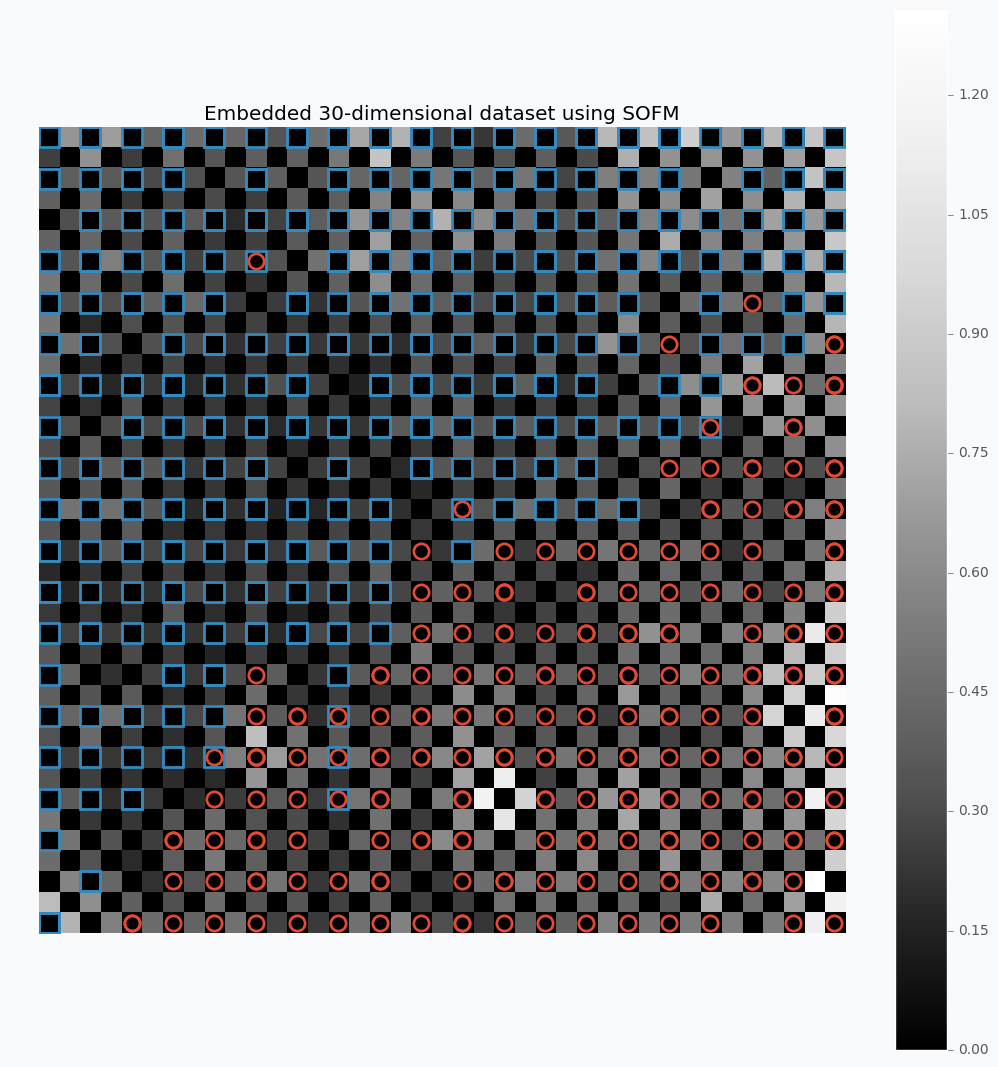
Now between every feature and its neighbor there is an extra square. As in the previous example each square encodes distance between two neighboring features. We do not consider two features in the map as neighbors in case if they connected diagonally. That’s why all diagonal squares between two micro-clusters color in black. Diagonals are a bit more difficult to encode, because in this case we have two different cases. In order to visualize it we can also take an average of these distances.
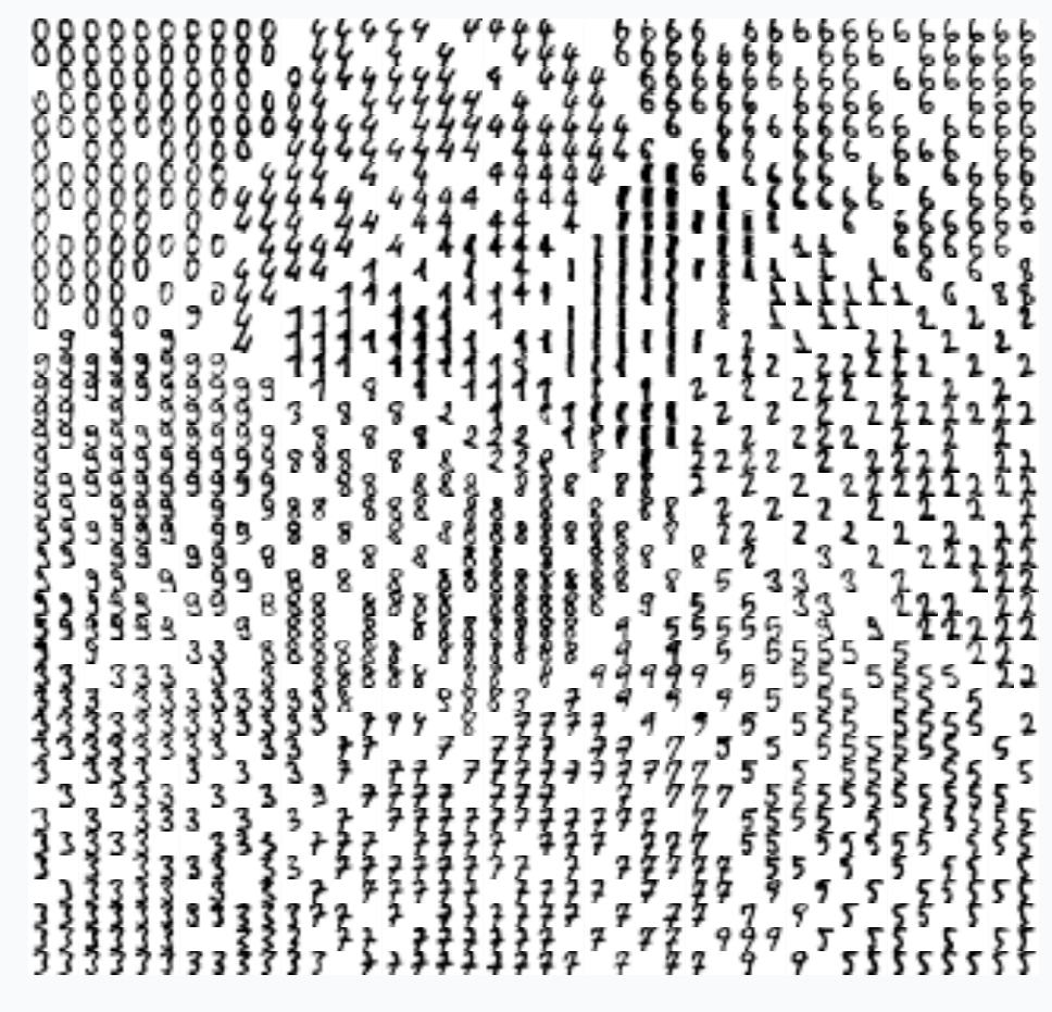
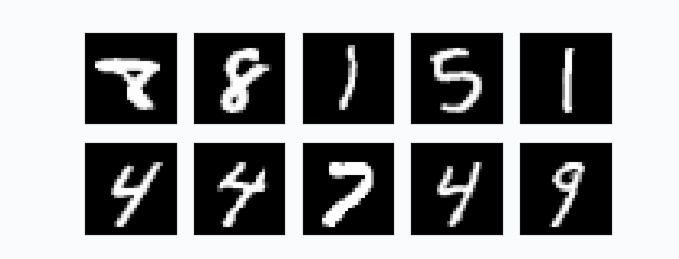
More interesting way to make this type of visualization can be with the use of images. In previous case, we use markers to encode two different classes. With images, we can use them directly as the way to represent the cluster. Let’s try to apply this idea on small dataset with images of digits from 0 to 9.
$ python sofm_digits.py
Visualize pre-trained VGG19 network
Using the same techniques, we can look inside the deep neural networks. In this section, I will be looking on the pre-trained VGG19 network using ImageNet data. Only in this case, I decided to make it a bit more challenging. Instead of using data from ImageNet I decided to pick 9 classes of different animal species from Caltech 101 dataset. The interesting part is that there are a few species that are not in the ImageNet.
The goal for this visualization is not only to see how the VGG19 network will separate different classes, but also to see if it would be able to extract some special features of the new classes that it hasn’t seen before. This information can be useful for the Transfer Learning, because from the visualization we should be able to see if network can separate unknown class from the other. If it will then it means there is no need to re-train all layers below the one which we are visualizing.
From the Caltech 101 dataset I picked the following classes:

There are a few classes that hasn’t been used in ImageNet, namely Okapi, Wild cat and Platypus.
Data was prepared in the same way as it was done for the VGG19 during training on ImageNet data. I first removed final layer from the network. Now output for each image should be 4096-dimensional vector. Because of the large dimensional size, I used cosine similarity in order to find closest SOFM neurons (instead of euclidian which we used in all previous examples).
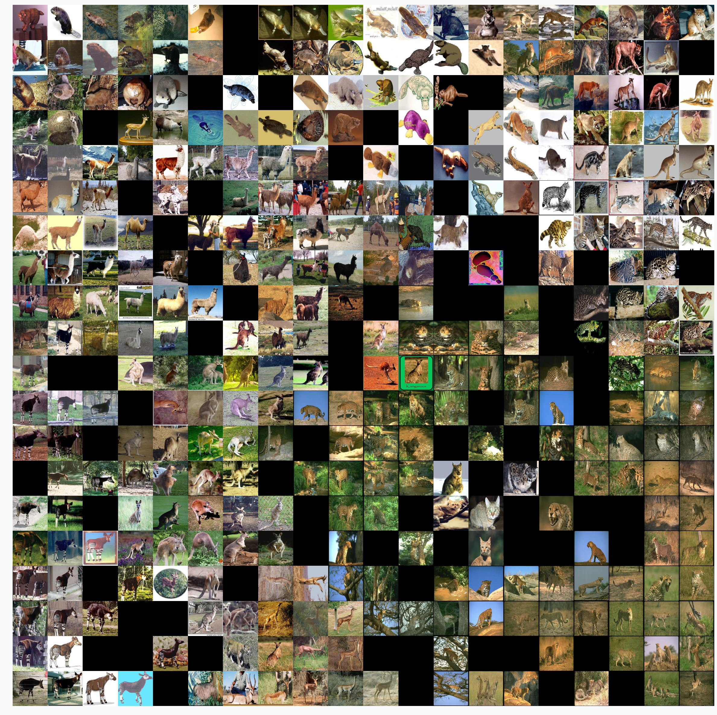
Even without getting into the details it’s easy to see that SOFM produces pretty meaningful visualization. Similar species are close to each other in the visualization which means that the main properties was captured correctly.
We can also visualize output from the last layer. From the network, we only need to remove final Softmax layer in order to get raw activation values. Using this values, we can also visualize our data.
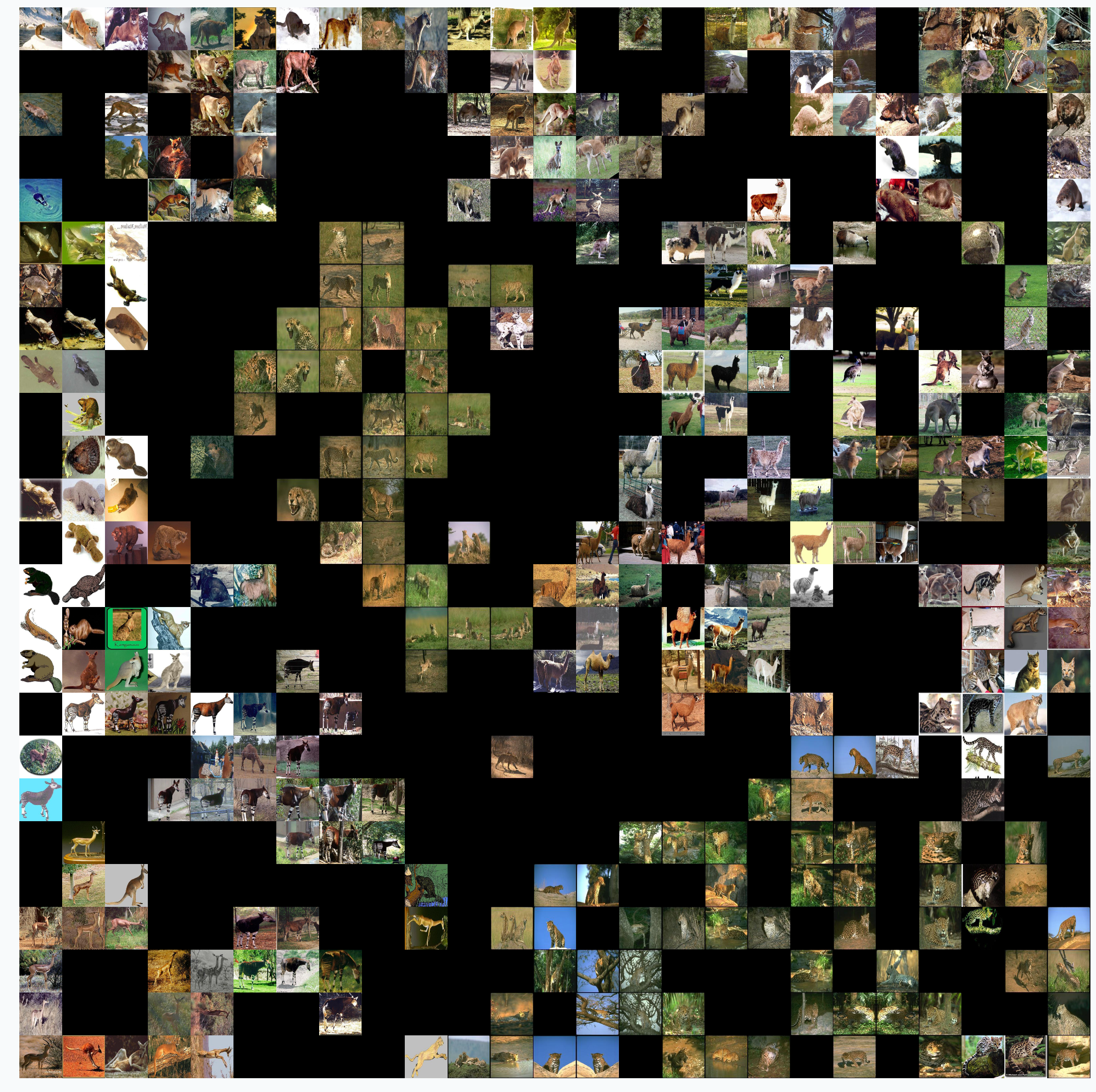
SOFM managed to identify high-dimensional structure pretty good. There are many interesting things that we can gain from this image. For instance, beaver and platypus share similar features. Since platypus wasn’t a part of the ImageNet dataset it is a reasonable mistake for the network to mix these species.
You probably noticed that there are many black squares in the image. Each square represents a gap between two micro-clusters. You can see how images of separate species are separated from other species with these gaps.
You can also see that network learned to classify rotated and scaled images very similarly which tells us that it is robust against small transformations applied to the image. In the image below, we can see a few examples.
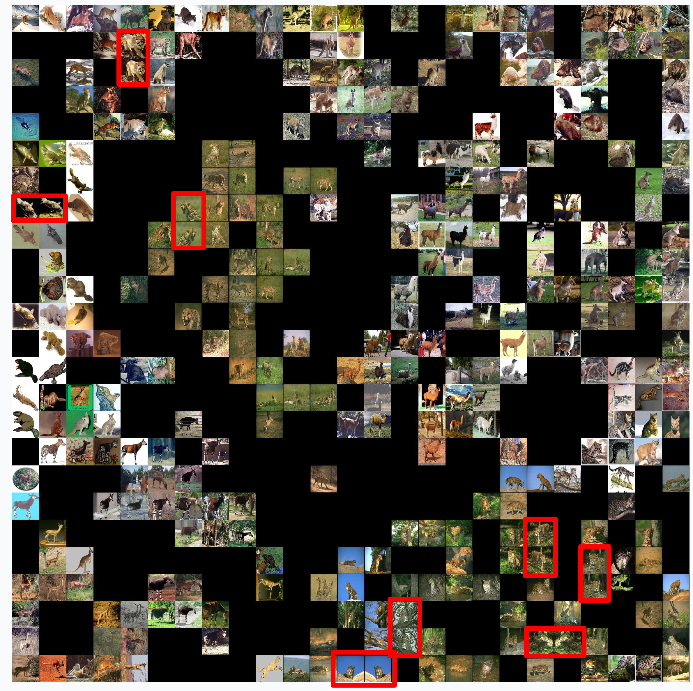
There are also some things that shows us problems with VGG19 network.. For instance, look at the image of llama that really close to the cheetah’s images.

This image looks out of place. We can check top 5 classes based on the probability that network gives to this image.
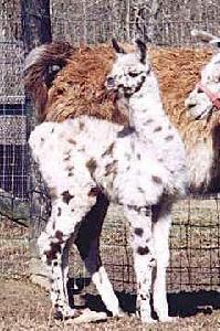
llama                                    : 31.18%
cheetah, chetah, Acinonyx jubatus        : 22.62%
tiger, Panthera tigris                   : 8.20%
lynx, catamount                          : 7.34%
snow leopard, ounce, Panthera uncia      : 5.91%
Prediction is correct, but look at the second choice. Percentage that it might be a cheetah is also pretty high. Even though cheetah and llama species are not very similar to each other, network still thinks that it can be a cheetah. The most obvious explanation of this phenomena is that llama in the image covered with spots all over the body which is a typical feature for cheetah. This example shows how easily we can fool the network.
Summary
In the article, I mentioned a few applications where SOFM can be used, but it’s not the full list. It can be also used for other applications like robotics or even for creating some beautiful pictures. It is fascinating how such a simple set of rules can be applied in order to solve very different problems.
Despite all the positive things that can be said about SOFM there are some problems that you encounter.
- There are many hyperparameters and selecting the right set of parameter can be tricky.
- SOFM doesn’t cover borders of the dataspace which means that area, volume or hypervolume of the data will be smaller than it is in real life. You can see it from the picture where we approximate circles.
It also means that if you need to pick information about outliers from your data - SOFM will probably miss it.
- Not every space approximates with SOFM. There can be some cases where SOFM fits data poorly which sometimes difficult to see.
Code
iPython notebook with code that explores VGG19 using SOFM available on github. NeuPy has Python scripts that can help you to start work with SOFM or show you how you can use SOFM for different applications.
- Simple SOFM example
- Clustering iris dataset using SOFM
- Learning half-circle topology with SOFM
- Compare feature grid types for SOFM
- Compare weight initialization methods for SOFM
- Visualize digit images in 2D space with SOFM
- Embedding 30-dimensional dataset into 2D and building heatmap visualization for SOFM
Hyperparameter optimization for Neural Networks
Contents
Introduction
Sometimes it can be difficult to choose a correct architecture for Neural Networks. Usually, this process requires a lot of experience because networks include many parameters. Let’s check some of the most important parameters that we can optimize for the neural network:
- Number of layers
- Different parameters for each layer (number of hidden units, filter size for convolutional layer and so on)
- Type of activation functions
- Parameter initialization method
- Learning rate
- Loss function
Even though the list of parameters in not even close to being complete, it’s still impressive how many parameters influences network’s performance.
Hyperparameter optimization
In this article, I would like to show a few different hyperparameter selection methods.
- Grid Search
- Random Search
- Hand-tuning
- Gaussian Process with Expected Improvement
- Tree-structured Parzen Estimators (TPE)
Grid Search
The simplest algorithms that you can use for hyperparameter optimization is a Grid Search. The idea is simple and straightforward. You just need to define a set of parameter values, train model for all possible parameter combinations and select the best one. This method is a good choice only when model can train quickly, which is not the case for typical neural networks.
Imagine that we need to optimize 5 parameters. Let’s assume, for simplicity, that we want to try 10 different values per each parameter. Therefore, we need to make 100,000 (\(10 ^ 5\)) evaluations. Assuming that network trains 10 minutes on average we will have finished hyperparameter tuning in almost 2 years. Seems crazy, right? Typically, network trains much longer and we need to tune more hyperparameters, which means that it can take forever to run grid search for typical neural network. The better solution is random search.
Random Search
The idea is similar to Grid Search, but instead of trying all possible combinations we will just use randomly selected subset of the parameters. Instead of trying to check 100,000 samples we can check only 1,000 of parameters. Now it should take a week to run hyperparameter optimization instead of 2 years.
Let’s sample 100 two-dimensional data points from a uniform distribution.
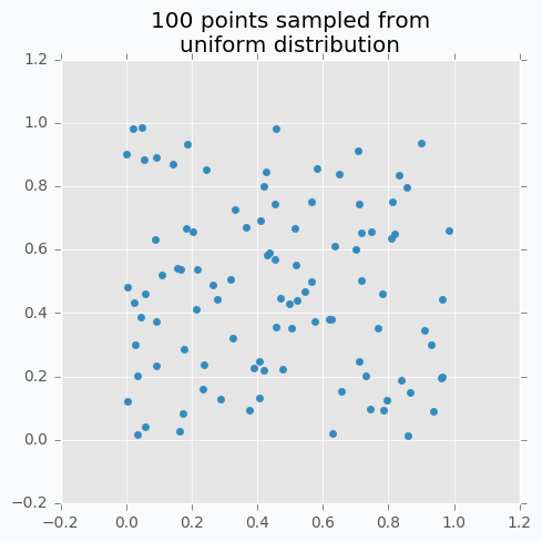
In case if there are not enough data points, random sampling doesn’t fully covers parameter space. It can be seen in the figure above because there are some regions that don’t have data points. In addition, it samples some points very close to each other which are redundant for our purposes. We can solve this problem with Low-discrepancy sequences (also called quasi-random sequences).
There are many different techniques for quasi-random sequences:
- Sobol sequence
- Hammersley set
- Halton sequence
- Poisson disk sampling
Let’s compare some of the mentioned methods with previously random sampled data points.
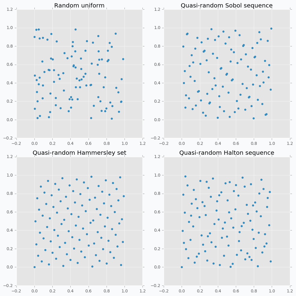
As we can see now sampled points spread out through the parameter space more uniformly. One disadvantage of these methods is that not all of them can provide you good results for the higher dimensions. For instance, Halton sequence and Hammersley set do not work well for dimension bigger than 10 [7].
Even though we improved hyperparameter optimization algorithm it still is not suitable for large neural networks.
But before we move on to more complicated methods I want to focus on parameter hand-tuning.
Hand-tuning
Let’s start with an example. Imagine that we want to select the best number of units in the hidden layer (we set up just one hyperparameter for simplicity). The simplest thing is to try different values and select the best one. Let’s say we set up 10 units for the hidden layer and train the network. After the training, we check the accuracy for the validation dataset and it turns out that we classified 65% of the samples correctly.
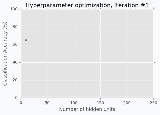
The accuracy is low, so it’s intuitive to think that we need more units in a hidden layer. Let’s increase the number of units and check the improvement. But, by how many should we increase the number of units? Will small changes make a significant effect on the prediction accuracy? Would it be a good step to set up a number of hidden units equal to 12? Probably not. So let’s go further and explore parameters from the next order of magnitude. We can set up a number of hidden units equal to 100.
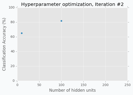
For the 100 hidden units, we got prediction accuracy equal to 82% which is a great improvement compared to 65%. Two points in the figure above show us that by increasing number of hidden units we increase the accuracy. We can proceed using the same strategy and train network with 200 hidden units.

After the third iteration, our prediction accuracy is 84%. We’ve increased the number of units by a factor of two and got only 2% of improvement.
We can keep going, but I think judging by this example it is clear that human can select parameters better than Grid search or Random search algorithms. The main reason why is that we are able to learn from our previous mistakes. After each iteration, we memorize and analyze our previous results. This information gives us a much better way for selection of the next set of parameters. And even more than that. The more you work with neural networks the better intuition you develop for what and when to use.
Nevertheless, let’s get back to our optimization problem. How can we automate the process described above? One way of doing this is to apply a Bayesian Optimization.
Bayesian Optimization
Bayesian optimization is a derivative-free optimization method. There are a few different algorithm for this type of optimization, but I was specifically interested in Gaussian Process with Acquisition Function. For some people it can resemble the method that we’ve described above in the Hand-tuning section. Gaussian Process uses a set of previously evaluated parameters and resulting accuracy to make an assumption about unobserved parameters. Acquisition Function using this information suggest the next set of parameters.
Gaussian Process
The idea behind Gaussian Process is that for every input \(x\) we have output \(y = f(x)\), where \(f\) is a stochastic function. This function samples output from a gaussian distribution. Also, we can say that each input \(x\) has associated gaussian distribution. Which means that for each input \(x\) gaussian process has defined mean \(\mu\) and standard deviation \(\sigma\) for some gaussian distribution.
Gaussian Process is a generalization of Multivariate Gaussian Distribution. Multivariate Gaussian Distribution is defined by mean vector and covariance matrix, while Gaussian Process is defined by mean function and covariance function. Basically, a function is an infinite vector. Also, we can say that Multivariate Gaussian Distribution is a Gaussian Process for the functions with a discrete number of possible inputs.
I always like to have some picture that shows me a visual description of an algorithm. One of such visualizations of the Gaussian Process I found in the Introduction to Gaussian Process slides [3].
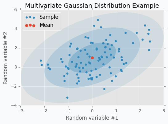
Let’s check some Multivariate Gaussian Distribution defined by mean vector \(\mu\)
and covariance matrix \(\Sigma\)
We can sample 100 points from this distribution and make a scatter plot.
Another way to visualize these samples might be Parallel Coordinates.
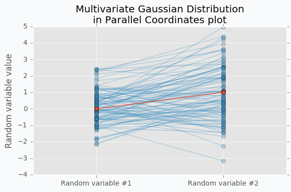
You should understand that lines that connect points are just an imaginary relations between each coordinate. There is nothing in between Random variable #1 and Random variable #2.
An interesting thing happens when we increase the number of samples.

Now we can see that lines form a smooth shape. This shape defines a correlation between two random variables. If it’s very narrow in the middle then there is a negative correlation between two random variables.
With scatter plot we are limited to numbers of dimensions that we can visualize, but with Parallel Coordinates we can add more dimensions. Let’s define new Multivariate Gaussian Distribution using 5 random variables.
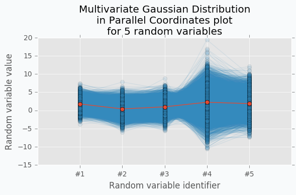
With more variables, it looks more like a function. We can increase the number of dimensions and still be able to visualize Multivariate Gaussian Distribution. The more dimensions we add the more it looks like a set of functions sampled from the Gaussian Process. But in case of Gaussian Process number of dimensions should be infinite.
Let’s get data from the Hand-tuning section (the one where with 10 hidden units we got 65% of accuracy). Using this data we can train Gaussian Process and predict mean and standard deviation for each point \(x\).

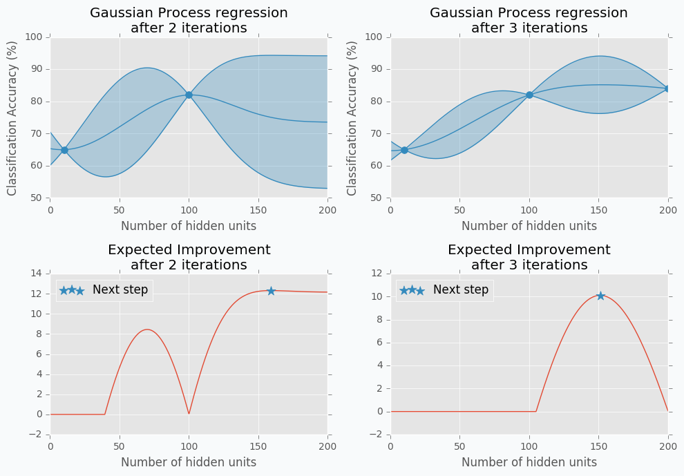
The blue region defines 95% confidence interval for each point \(x\). It’s easy to see that the further we go from the observed samples the wider confidence interval becomes which is a logical conclusion. The opposite is true as well. Very similar to the logic that a person uses to select next set of parameters.
From the plot, it looks like observed data points doesn’t have any variance. In fact, the variance is not zero, it’s just really tiny. That’s because our previous Gaussian Process configuration is expecting that our prediction was obtained from a deterministic function which is not true for most neural networks. To fix it we can change the parameter for the Gaussian Process that defines the amount of noise in observed variables. This trick will not only give us a prediction that is less certain but also a mean of the number of hidden units that won’t go through the observed data points.

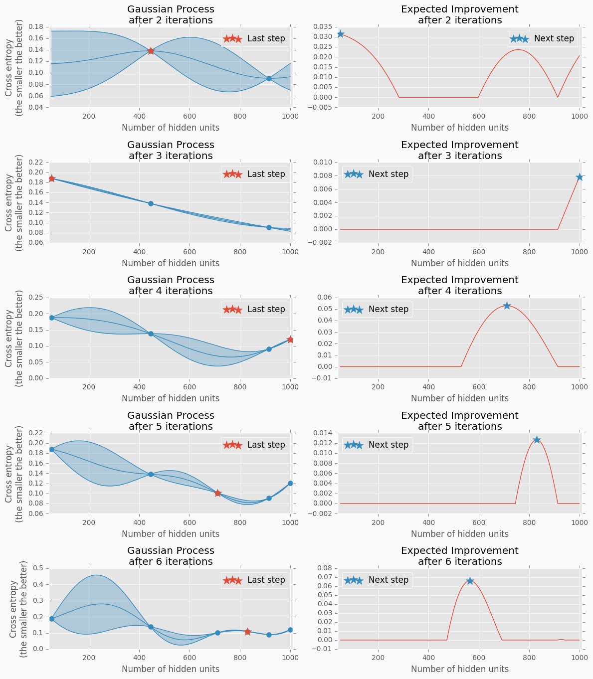
Acquisition Function
Acquisition Function defines the set of parameter for our next step. There are many different functions [1] that can help us calculate the best value for the next step. One of the most common is Expected Improvement. There are two ways to compute it. In case if we are trying to find minimum we can use this formula.
where \(y_{min}\) is the minimum observed value \(y\) and \(y_{lowest\ expected}\) lowest possible value from the confidence interval associated with each possible value \(x\).
In our case, we are trying to find the maximum value. With the small modifications, we can change last formula in the way that will identify Expected Improvement for the maximum value.
where \(y_{max}\) is the maximum observed value and \(y_{highest\ expected}\) highest possible value from the confidence interval associated with each possible value \(x\).
Here is an output for each point \(x\) for the Expected Improvement function.
Disadvantages of GP with EI
There are a few disadvantages related to the Gaussian Process with Expected Improvement.
- It doesn’t work well for categorical variables. In case if neural networks it can be a type of activation function.
- GP with EI selects new set of parameters based on the best observation. Neural Network usually involves randomization (like weight initialization and dropout) during the training process which influences a final score. Running neural network with the same parameters can lead to different scores. Which means that our best score can be just lucky output for the specific set of parameters.
- It can be difficult to select right hyperparameters for Gaussian Process. Gaussian Process has lots of different kernel types. In addition you can construct more complicated kernels using simple kernels as a building block.
- It works slower when number of hyperparameters increases. That’s an issue when you deal with a huge number of parameters.
Tree-structured Parzen Estimators (TPE)
Overview
Tree-structured Parzen Estimators (TPE) fixes disadvantages of the Gaussian Process. Each iteration TPE collects new observation and at the end of the iteration, the algorithm decides which set of parameters it should try next. The main idea is similar, but an algorithm is completely different
At the very beginning, we need to define a prior distribution for out hyperparameters. By default, they can be all uniformly distributed, but it’s possible to associate any hyperparameter with some random unimodal distribution.
For the first few iterations, we need to warn up TPE algorithm. It means that we need to collect some data at first before we can apply TPE. The best and simplest way to do it is just to perform a few iterations of Random Search. A number of iterations for Random Search is a parameter defined by the user for the TPE algorithm.
When we collected some data we can finally apply TPE. The next step is to divide collected observations into two groups. The first group contains observations that gave best scores after evaluation and the second one - all other observations. And the goal is to find a set of parameters that more likely to be in the first group and less likely to be in the second group. The fraction of the best observations is defined by the user as a parameter for the TPE algorithm. Typically, it’s 10-25% of observations.
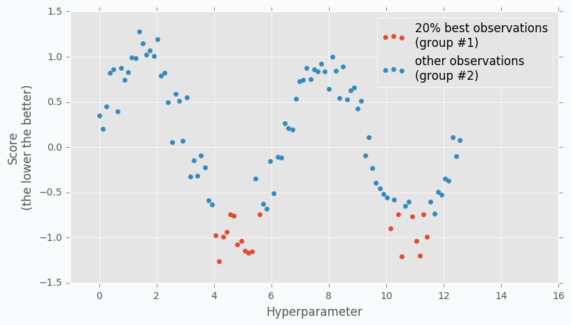
As you can see we are no longer rely on the best observation. Instead, we use a distribution of the best observations. The more iterations we use during the Random Search the better distribution we have at the beginning.
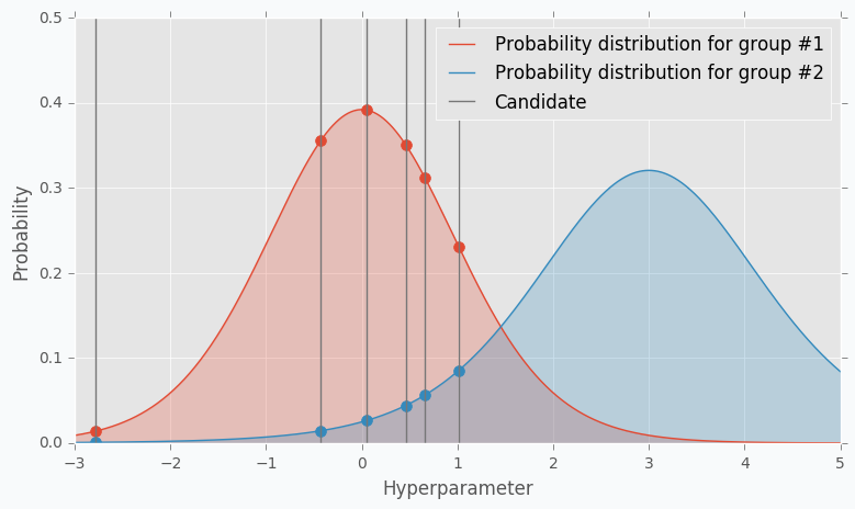
The next part of the TPE is to model likelihood probability for each of the two groups. This is the next big difference between Gaussian Process and TPE. For Gaussian Process we’ve modeled posterior probability instead of likelihood probability. Using the likelihood probability from the first group (the one that contains best observations) we sample the bunch of candidates. From the sampled candidates we try to find a candidate that more likely to be in the first group and less likely to be in the second one. The following formula defines Expected Improvement per each candidate.
Where \(l(x)\) is a probability being in the first group and \(g(x)\) is a probability being in the second group.
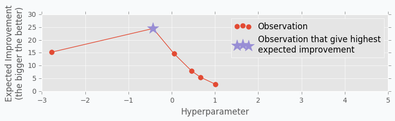
Here is an example. Let’s say we have predefined distribution for both groups. From the group #1, we sample 6 candidates. And for each, we calculate Expected Improvement. A parameter that has the highest improvement is the one that we will use for the next iteration.
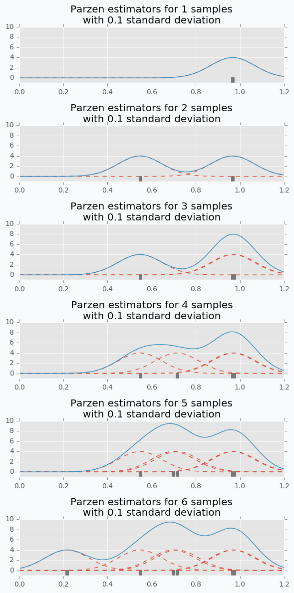
In the example, I’ve used t-distributions, but in TPE distribution models using parzen-window density estimators. The main idea is that each sample defines gaussian distribution with specified mean (value of the hyperparameter) and standard deviation. Then all these points stacks together and normalized to assure that output is Probability Density Function (PDF). That’s why Parzen estimators appears in the name of the algorithm.
And the tree-structured means that parameter space defines in a form of a tree. Later we will try to find the best number of layers for the network. In our case, we will try to decide whether it’s better to use one or two hidden layers. In case if we use two hidden layers we should define the number of hidden units for the first and second layer independently. If we use one hidden layer we don’t need to define the number of hidden units for the second hidden layer, because it doesn’t exist for the specified set of parameter. Basically, it means that a number of hidden units in the second hidden layer depends on the number of hidden layers. Which means that parameters have tree-structured dependencies.
Hyperparameter optimization for MNIST dataset
Let’s make an example. We’re going to use MNIST dataset.
import numpy as np
from sklearn import datasets, preprocessing
from sklearn.model_selection import train_test_split

X, y = datasets.fetch_openml('mnist_784', version=1, return_X_y=True)

target_scaler = preprocessing.OneHotEncoder(sparse=False, categories='auto')
y = target_scaler.fit_transform(y.reshape(-1, 1))

X /= 255.
X -= X.mean(axis=0)

x_train, x_test, y_train, y_test = train_test_split(
    X.astype(np.float32),
    y.astype(np.float32),
    test_size=(1 / 7.)
)
For hyperparameter selection, I’m going to use hyperopt library. It has implemented TPE algorithm.
The hyperopt library gives the ability to define a prior distribution for each parameter. In the table below you can find information about parameters that we are going to tune.
| Parameter name | Distribution | Values |
|---|---|---|
| Step size | Log-uniform | \(x \in [0.01, 0.5]\) |
| Batch size | Log-uniform integer | \(x \in [16, 512]\) |
| Activation function | Categorical | \(x \in \{Relu, PRelu, Elu, Sigmoid, Tanh\}\) |
| Number of hidden layers | Categorical | \(x \in \{1, 2\}\) |
| Number of units in the first layer | Uniform integer | \(x \in [50, 1000]\) |
| Number of units in the second layer (In case if it defined) | Uniform integer | \(x \in [50, 1000]\) |
| Dropout layer | Uniform | \(x \in [0, 0.5]\) |
Here is one way to define our parameters in hyperopt.
import numpy as np
from hyperopt import hp

def uniform_int(name, lower, upper):
    # `quniform` returns:
    # round(uniform(low, high) / q) * q
    return hp.quniform(name, lower, upper, q=1)

def loguniform_int(name, lower, upper):
    # Do not forget to make a logarithm for the
    # lower and upper bounds.
    return hp.qloguniform(name, np.log(lower), np.log(upper), q=1)

parameter_space = {
    'step': hp.uniform('step', 0.01, 0.5),
    'layers': hp.choice('layers', [{
        'n_layers': 1,
        'n_units_layer': [
            uniform_int('n_units_layer_11', 50, 500),
        ],
    }, {
        'n_layers': 2,
        'n_units_layer': [
            uniform_int('n_units_layer_21', 50, 500),
            uniform_int('n_units_layer_22', 50, 500),
        ],
    }]),
    'act_func_type': hp.choice('act_func_type', [
        layers.Relu,
        layers.PRelu,
        layers.Elu,
        layers.Tanh,
        layers.Sigmoid
    ]),

    'dropout': hp.uniform('dropout', 0, 0.5),
    'batch_size': loguniform_int('batch_size', 16, 512),
}
I won’t get into details. I think that definitions are pretty clear from the code. In case if you want to learn more about hyperopt parameter space initialization you can check this link.
Next we need to construct a function that we want to minimize. In our case function should train network using training dataset and return cross entropy error for validation dataset.
from pprint import pprint

def train_network(parameters):
    print("Parameters:")
    pprint(parameters)
    print()
First of all, in the training function, we need to extract our parameter.
step = parameters['step']
batch_size = int(parameters['batch_size'])
proba = parameters['dropout']
activation_layer = parameters['act_func_type']
layer_sizes = [int(n) for n in parameters['layers']['n_units_layer']]
Note that some of the parameters I converted to the integer. The problem is that hyperopt returns float types and we need to convert them.
Next, we need to construct network based on the presented information. In our case, we use only one or two hidden layers, but it can be any arbitrary number of layers.
from neupy import layers

network = layers.Input(784)

for layer_size in layer_sizes:
    network = network >> activation_layer(layer_size)

network = network >> layers.Dropout(proba) >> layers.Softmax(10)
To learn more about layers in NeuPy you should check documentation.
After that, we can define training algorithm for the network.
from neupy import algorithms
from neupy.exceptions import StopTraining

def on_epoch_end(network):
    if network.training_errors[-1] > 10:
        raise StopTraining("Training was interrupted. Error is to high.")

mnet = algorithms.RMSProp(
    network,

    batch_size=batch_size,
    step=step,

    loss='categorical_crossentropy',
    shuffle_data=True,

    signals=on_epoch_end,
)
All settings should be clear from the code. You can check RMSProp documentation to find more information about its input parameters. In addition, I’ve added a simple rule that interrupts training when the error is too high. This is an example of a simple rule that can be changed.
Now we can train our network.
mnet.train(x_train, y_train, epochs=50)
And at the end of the function, we can check some information about the training progress.
score = mnet.score(x_test, y_test)

y_predicted = mnet.predict(x_test).argmax(axis=1)
accuracy = metrics.accuracy_score(y_test.argmax(axis=1), y_predicted)

print("Final score: {}".format(score))
print("Accuracy: {:.2%}".format(accuracy))

return score
You can see that I’ve used two evaluation metrics. First one is cross-entropy. NeuPy uses it as a validation error function when we call the score method. The second one is just a prediction accuracy.
And finally, we run hyperparameter optimization.
import hyperopt
from functools import partial

# Object stores all information about each trial.
# Also, it stores information about the best trial.
trials = hyperopt.Trials()

tpe = partial(
    hyperopt.tpe.suggest,

    # Sample 1000 candidate and select candidate that
    # has highest Expected Improvement (EI)
    n_EI_candidates=1000,

    # Use 20% of best observations to estimate next
    # set of parameters
    gamma=0.2,

    # First 20 trials are going to be random
    n_startup_jobs=20,
)

hyperopt.fmin(
    train_network,

    trials=trials,
    space=parameter_space,

    # Set up TPE for hyperparameter optimization
    algo=tpe,

    # Maximum number of iterations. Basically it trains at
    # most 200 networks before selecting the best one.
    max_evals=200,
)
And after all trials, we can check the best one in the trials.best_trial attribute.
Disadvantages of TPE
On of the biggest disadvantages of this algorithm is that it selects parameters independently from each other. For instance, there is a clear relation between regularization and number of training epoch parameters. With regularization, we usually can train network for more epochs and with more epochs we can achieve better results. On the other hand without regularization, many epochs can be a bad choice because network starts overfitting and validation error increases. Without taking into account the state of the regularization variable each next choice for the number of epochs can look arbitrary.
It’s good in case if you now that some variables have relations. To overcome problem from the previous example you can construct two different choices for epochs. The first one will enable regularization and selects a number of epochs from the \([500, 1000]\) range. And the second one without regularization and selects number of epochs from the \([10, 200]\) range.
hp.choice('training_parameters', [
    {
        'regularization': True,
        'n_epochs': hp.quniform('n_epochs', 500, 1000, q=1),
    }, {
        'regularization': False,
        'n_epochs': hp.quniform('n_epochs', 20, 300, q=1),
    },
])
Summary
The Bayesian Optimization and TPE algorithms show great improvement over the classic hyperparameter optimization methods. They allow to learn from the training history and give better and better estimations for the next set of parameters. But it still takes lots of time to apply these algorithms. It’s great if you have an access to multiple machines and you can parallel parameter tuning procedure [4], but usually, it’s not an option. Sometimes it’s better just to avoid hyperparameter optimization. In case if you just try to build a network for trivial problems like image classification it’s better to use existed architectures with pre-trained parameters like VGG19 or ResNet.
For unique problems that don’t have pre-trained networks the classic and simple hand-tuning is a great way to start. A few iterations can give you a good architecture which won’t be the state-of-the-art but should give you satisfying result with a minimum of problems. In case if accuracy does not suffice your needs you can always boost your performance getting more data or developing ensembles with different models.
Source Code
All source code is available on GitHub in the iPython notebook. It includes all visualizations and hyperparameter selection algorithms.
References
| [1] | Bayesian Optimization and Acquisition Functions from http://www.cse.wustl.edu/~garnett/cse515t/files/lecture_notes/12.pdf |
| [2] | Gaussian Processes in Machine Learning from http://mlg.eng.cam.ac.uk/pub/pdf/Ras04.pdf |
| [3] | Slides: Introduction to Gaussian Process from https://www.cs.toronto.edu/~hinton/csc2515/notes/gp_slides_fall08.pdf |
| [4] | Preliminary Evaluation of Hyperopt Algorithms on HPOLib from http://compneuro.uwaterloo.ca/files/publications/bergstra.2014.pdf |
| [5] | Algorithms for Hyper-Parameter Optimization from http://papers.nips.cc/paper/4443-algorithms-for-hyper-parameter-optimization.pdf |
| [6] | Slides: Pattern Recognition, Lecture 6 from http://www.csd.uwo.ca/~olga/Courses/CS434a_541a/Lecture6.pdf |
| [7] | Low-discrepancy sampling methods from http://planning.cs.uiuc.edu/node210.html |
| [8] | Parzen-Window Density Estimation from https://www.cs.utah.edu/~suyash/Dissertation_html/node11.html |
Image classification, MNIST digits
This short tutorial shows how to build and train simple network for digit classification in NeuPy.
Data preparation
Data can be loaded in different ways. I used scikit-learn to fetch the MNIST dataset.
>>> from sklearn import datasets
>>> X, y = datasets.fetch_openml('mnist_784', version=1, return_X_y=True)
Now that we have the data we need to confirm that we have expected number of samples.
>>> X.shape
(70000, 784)
>>> y.shape
(70000,)
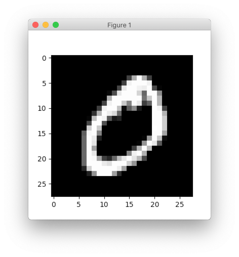
Every data sample has 784 features and they can be reshaped into 28x28 image.
>>> import matplotlib.pyplot as plt
>>> plt.imshow(X[0].reshape((28, 28)), cmap='gray')
>>> plt.show()
In this tutorial, we will use each image as a vector so we won’t need to reshape it to its original size. The only thing that we need to do is to rescale image values. Rescaling images will help network to converge faster.
>>> X = X.astype(np.float32)
>>> X /= 255.
>>> X -= X.mean(axis=0)
Notice the way division and subtraction are specified. In this way, we make update directly on the X matrix without copying it. It can be validated with simple example.
>>> import numpy as np
>>> A = np.random.random((100, 10))
>>> id(A)  # numbers will be different between runs
4486892960
>>>
>>> A -= 3
>>> id(A)  # object ID didn't change
4486892960
>>>
>>> A = A - 3
>>> id(A)  # and now it's different, because it's different object
4602409968
After last update for matrix A we got different identifier for the object, which means that it got copied.
In case of the in-place updates, we don’t waste memory. Current dataset is relatively small and there is no memory deficiency, but for larger datasets it might make a big difference.
There is one more processing step that we need to do before we can train our network. Let’s take a look into target classes.
>>> import random
>>> random.sample(y.astype('int').tolist(), 10)
[9, 0, 9, 7, 2, 2, 3, 0, 0, 8]
All the numbers that we have are specified as integers. For our problem we want network to learn visual representation of the numbers. We cannot use them as integers, because it will create problems during the training. Basically, with the integer definition we’re implying that number 1 visually more similar to 0 than to number 7. It happens only because difference between 1 and 0 smaller than difference between 1 and 7. In order to avoid making any type of assumptions we will use one-hot encoding technique.
>>> from sklearn.preprocessing import OneHotEncoder
>>> encoder = OneHotEncoder(sparse=False)
>>> y = encoder.fit_transform(y.reshape(-1, 1))
>>> y.shape
(70000, 10)
You can see that every digit was transformed into a 10 dimensional vector.
And finally, we need to divide our data into training and validation set. We won’t show validation set to the network and we will use it only to test network’s classification accuracy.
>>> import numpy as np
>>> from sklearn.model_selection import train_test_split
>>>
>>> x_train, x_test, y_train, y_test = train_test_split(
...     X.astype(np.float32),
...     y.astype(np.float32),
...     test_size=(1 / 7.)
... )
Notice that data was converted into 32 bit float numbers. This is the only float type that currently supported by NeuPy.
Model initialization
It’s very easy to define neural network architectures in the NeuPy. We can define simple architecture that excepts input vector with 784 features and outputs probabilities per each digit class. In addition, we can two hidden layers with 500 and 300 output units respectively. Each hidden layer will use relu as activation function
from neupy.layers import *

network = join(
    # Every image in the MNIST dataset has 784 pixels (28x28)
    Input(784),

    # Hidden layers
    Relu(500),
    Relu(300),

    # Softmax layer ensures that we output probabilities
    # and specified number of outputs equal to the unique
    # number of classes
    Softmax(10),
)
Because our neural network is quite small, we can rewrite this architecture with a help of the inline operator.
network = Input(784) >> Relu(500) >> Relu(300) >> Softmax(10)
Now that we have our architecture we can initialize training algorithm.
from neupy import algorithms

optimizer = algorithms.Momentum(
    network,

    # Categorical cross-entropy is very popular loss function
    # for the multi-class classification problems
    loss='categorical_crossentropy',

    # Number of samples propagated through the network
    # before every weight update
    batch_size=128,

    # Learning rate
    step=0.01,

    # Makes sure that training progress will be
    # printed in the terminal
    verbose=True,

    # Training data will be shuffled before every epoch
    # It ensures that every batch will have different number of samples
    shuffle_data=True,

    # Options specific for the momentum training algorithm
    momentum=0.99,
    nesterov=True,
)
All the most important information related to the neural network you can find in the terminal output. If you run the code that shown above you should see output similar to the one shown below.
Main information

[ALGORITHM] Momentum

[OPTION] batch_size = 128
[OPTION] loss = categorical_crossentropy
[OPTION] momentum = 0.99
[OPTION] nesterov = True
[OPTION] regularizer = None
[OPTION] show_epoch = 1
[OPTION] shuffle_data = True
[OPTION] signals = None
[OPTION] step = 0.01
[OPTION] target = Tensor("placeholder/target/softmax-9:0", shape=(?, 10), dtype=float32)
[OPTION] verbose = True

[TENSORFLOW] Initializing Tensorflow variables and functions.
[TENSORFLOW] Initialization finished successfully. It took 0.47 seconds
Training
Now that we have everything specified we are finally can train our network. In addition, we can add test data for which we will be able to monitor network’s training progress on the unseen data.
>>> optimizer.train(x_train, y_train, x_test, y_test, epochs=10)
#1 : [2 sec] train: 0.124558, valid: 0.123087
#2 : [2 sec] train: 0.011129, valid: 0.079253
#3 : [2 sec] train: 0.052001, valid: 0.081510
#4 : [2 sec] train: 0.008683, valid: 0.071755
#5 : [2 sec] train: 0.033496, valid: 0.076705
#6 : [2 sec] train: 0.002223, valid: 0.073506
#7 : [2 sec] train: 0.002255, valid: 0.076624
#8 : [2 sec] train: 0.036734, valid: 0.080020
#9 : [2 sec] train: 0.000858, valid: 0.076834
#10 : [2 sec] train: 0.001999, valid: 0.078267
Evaluations
From the table it’s hard to see network’s training progress. We can make error plot that can help us to visualize how it performed on the training and validation datasets separately.
>>> optimizer.plot_errors()
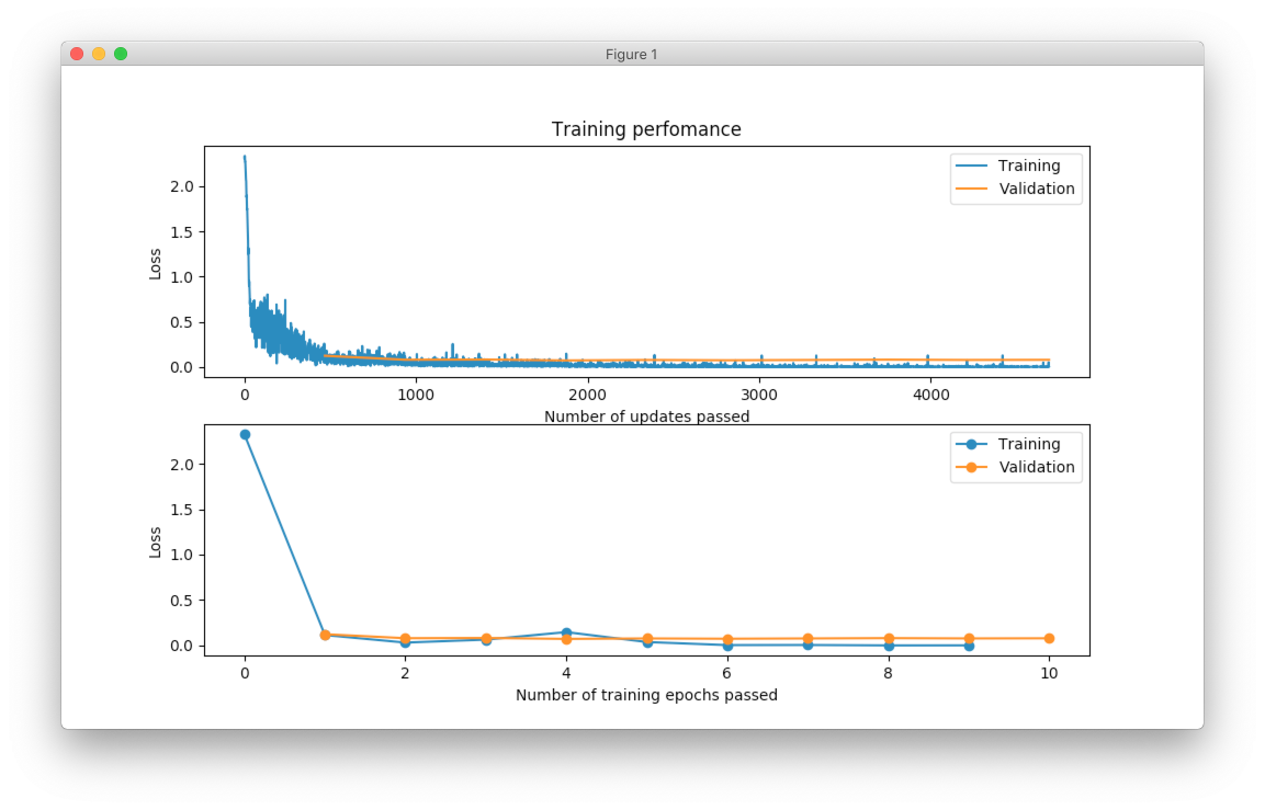
From the figure above, you can notice that validation error does not decrease all the time. Sometimes it goes up and sometimes down, but it doesn’t mean that network trains poorly. Let’s check small example that can explain who it can happen.
>>> actual_values = np.array([1, 1, 0])
>>> model1_prediction = np.array([0.9, 0.9, 0.6])
>>> model2_prediction = np.array([0.6, 0.6, 0.4])
Above, you can see two predictions from different models. The first model predicted two samples right and one wrong. The second one predicted everything perfectly, but predictions from second model are less certain (probabilities are close to random prediction - 0.5). Let’s check the binary cross entropy error.
>>> from sklearn.metrics import log_loss as binary_crossentropy
>>> binary_crossentropy(actual_values, model1_prediction)
0.37567
>>> binary_crossentropy(actual_values, model2_prediction)
0.51083
The second model made better prediction in terms of accuracy, but it got larger cross entropy error. Larger error means that network is less certain about its prediction. Similar situation we’ve observed in the plot above.
Instead of using cross-entropy error for model performance assessment we can build our own report using functions available in scikit-learn library.
>>> from sklearn import metrics
>>>
>>> y_predicted = optimizer.predict(x_test).argmax(axis=1)
>>> y_actual = np.asarray(y_test.argmax(axis=1)).reshape(len(y_test))
>>>
>>> print(metrics.classification_report(y_actual, y_predicted))
              precision    recall  f1-score   support

           0       0.99      0.99      0.99       972
           1       0.99      0.99      0.99      1130
           2       0.99      0.98      0.98       997
           3       0.99      0.98      0.98      1061
           4       0.97      0.99      0.98       966
           5       0.98      0.98      0.98       865
           6       0.99      0.99      0.99      1029
           7       0.98      0.99      0.98      1017
           8       0.98      0.98      0.98       952
           9       0.97      0.98      0.98      1011

   micro avg       0.98      0.98      0.98     10000
   macro avg       0.98      0.98      0.98     10000
weighted avg       0.98      0.98      0.98     10000

>>> score = metrics.accuracy_score(y_actual, y_predicted)
>>> print("Validation accuracy: {:.2%}".format(score))
Validation accuracy: 98.37%
The 98.37% accuracy is pretty good accuracy for such a simple solution. Additional modification can improve network’s accuracy.
Password recovery
Contents
In this article we are going to build a simple neural network that will recover password from a broken one. If you aren’t familiar with a Discrete Hopfield Network algorithm, you can read this article.
Before running all experiments, we need to set up seed parameter to make all results reproducible. But you can test code without it.
from neupy import utils
utils.reproducible()
If you can’t reproduce with your version of Python or libraries you can install those ones that were used in this article:
>>> import neupy
>>> neupy.__version__
'0.3.0'
>>> import numpy
>>> numpy.__version__
'1.9.2'
>>> import platform
>>> platform.python_version()
'3.4.3'
Code works with a Python 2.7 as well.
Data transformation
Before building the network that will save and recover passwords, we should make transformations for input and output data. But it wouldn’t be enough just to encode it, we should set up a constant length for an input string to make sure that strings will have the same length Also we should define what string encoding we will use. For simplicity we will use only ASCII symbols. So, let’s define a function that transforms a string into a binary list.
def str2bin(text, max_length=30):
    if len(text) > max_length:
        raise ValueError("Text can't contains more "
                         "than {} symbols".format(max_length))

    text = text.rjust(max_length)

    bits_list = []
    for symbol in text:
        bits = bin(ord(symbol))
        # Cut `0b` from the beggining and fill with zeros if they
        # are missed
        bits = bits[2:].zfill(8)
        bits_list.extend(map(int, bits))

    return list(bits_list)
Our function takes 2 parameters. First one is the string that we want to encode. And second attribute is setting up a constant length for input vector. If length of the input string is less than max_length value, then function fills spaces at the beginning of the string.
Let’s check str2bin function output.
>>> str2bin("test", max_length=5)
[0, 0, 1, 0, 0, 0, 0, 0, 0, ... ]
>>> len(str2bin("test", max_length=5))
40
ASCII encoding uses 8 bits per symbol and we set up 5 symbols per string, so our vector length equals to 40. From the first output, as you can see, first 8 symbols are equal to 00100000, that is a space value from the ASCII table.
After preforming recovery procedure we will always be getting a binary list. So before we begin to store data in neural network, we should define another function that transforms a binary list back into a string (which is basically inversed operation to the previous function).
def chunker(sequence, size):
    for position in range(0, len(sequence), size):
        yield sequence[position:position + size]

def bin2str(array):
    characters = []
    for binary_symbol_code in chunker(array, size=8):
        binary_symbol_str = ''.join(map(str, binary_symbol_code))
        character = chr(int(binary_symbol_str, base=2))
        characters.append(character)
    return ''.join(characters).lstrip()
If we test this function we will get word test back.
>>> bin2str(str2bin("test", max_length=5))
'test'
Pay attention! Function has removed all spaces at the beggining of the string before bringing them back. We assume that password won’t contain space at the beggining.
Saving password into the network
Now we are ready to save the password into the network. For this task we are going to define another function that create network and save password inside of it. Let’s define this function and later we will look at it step by step.
import numpy as np
from neupy import algorithms

def save_password(real_password, noise_level=5):
    if noise_level < 1:
        raise ValueError("`noise_level` must be equal or greater than 1.")

    binary_password = str2bin(real_password)
    bin_password_len = len(binary_password)

    data = [binary_password]

    for _ in range(noise_level):
        # The farther from the 0.5 value the less likely
        # password recovery
        noise = np.random.binomial(1, 0.55, bin_password_len)
        data.append(noise)

    dhnet = algorithms.DiscreteHopfieldNetwork(mode='sync')
    dhnet.train(np.array(data))

    return dhnet
If you have already read Discrete Hopfield Network article, you should know that if we add only one vector into the network we will get it dublicated or with reversed signs through the whole matrix. To make it a little bit secure we can add some noise into the network. For this reason we introduce one additional parameter noise_level into the function. This parameter controls number of randomly generated binary vectors. With each iteration using Binomial distribution we generate random binary vector with 55% probability of getting 1 in noise vector. And then we put all the noise vectors and transformed password into one matrix. And finaly we save all data in the Discrete Hopfield Network.
And that’s it. Function returns trained network for a later usage.
But why do we use random binary vectors instead of the decoded random strings? The problem is in the similarity between two vectors. Let’s check two approaches and compare them with a Hamming distance. But before starting we should define a function that measures distance between two vectors.
import string
import random

def hamming_distance(left, right):
    left, right = np.array(left), np.array(right)
    if left.shape != right.shape:
        raise ValueError("Shapes must be equal")
    return (left != right).sum()

def generate_password(min_length=5, max_length=30):
    symbols = list(
        string.ascii_letters +
        string.digits +
        string.punctuation
    )
    password_len = random.randrange(min_length, max_length + 1)
    password = [np.random.choice(symbols) for _ in range(password_len)]
    return ''.join(password)
In addition you can see the generate_password function that we will use for tests. Let’s check Hamming distance between two randomly generate password vectors.
>>> hamming_distance(str2bin(generate_password(20, 20)),
...                  str2bin(generate_password(20, 20)))
70
As we can see two randomly generated passwords are very similar to each other (approximetly 70% (\(100 * (240 - 70) / 240\)) of bits are the same). But If we compare randomly generated password to random binary vector we will see the difference.
>>> hamming_distance(str2bin(generate_password(20, 20)),
...                  np.random.binomial(1, 0.55, 240))
134
Hamming distance is bigger than in the previous example. A little bit more than 55% of the bits are different.
The greater the difference between them the easier recovery procedure for the input vectors patterns from the network. For this reason we use randomly generated binary vector instead of random password.
Of course it’s better to save not randomly generated noise vectors but randomly generated passwords converted into binary vectors, cuz if you use wrong input pattern randomly generated password might be recovered instead of the correct one.
Recovering password from the network
Now we are going to define the last function which will recover a password from the network.
def recover_password(dhnet, broken_password):
    test = np.array(str2bin(broken_password))
    recovered_password = dhnet.predict(test)

    if recovered_password.ndim == 2:
        recovered_password = recovered_password[0, :]

    return bin2str(recovered_password)
Function takes two parameters. The first one is network example from which function will recover a password from a broken one. And the second parameter is a broken password.
Finnaly we can test password recovery from the network.
>>> my_password = "$My%Super^Secret*^&Passwd"
>>> dhnet = save_password(my_password, noise_level=12)
>>> recover_password(dhnet, "-My-Super-Secret---Passwd")
'$My%Super^Secret*^&Passwd'
>>> _ == my_password
True
>>>
>>> recover_password(dhnet, "-My-Super")
'\x19`\xa0\x04Í\x14#ÛE2er\x1eÛe#2m4jV\x07PqsCwd'
>>>
>>> recover_password(dhnet, "Invalid")
'\x02 \x1d`\x80$Ì\x1c#ÎE¢eò\x0eÛe§:/$ê\x04\x07@5sCu$'
>>>
>>> recover_password(dhnet, "MySuperSecretPasswd")
'$My%Super^Secret*^&Passwd'
>>> _ == my_password
True
Everithing looks fine. After multiple times code running you can rarely find a problem. Network can produce a string which wasn’t taught. This string can look almost like a password with a few different symbols. The problem appears when network creates additional local minimum somewhere between input patterns. We can’t prevent it from running into the local minimum. For more information about this problem you can check article about Discrete Hopfield Network.
Test it using Monte Carlo
Let’s test our solution with randomly generated passwords. For this task we can use Monte Carlo experiment. At each step we create random password and try to recover it from a broken password.
import pprint
from operator import itemgetter
from collections import OrderedDict

def cutword(word, k, fromleft=False):
    if fromleft:
        return (word[-k:] if k != 0 else '').rjust(len(word))
    return (word[:k] if k != 0 else '').ljust(len(word))

n_times = 10000
cases = OrderedDict([
    ('exclude-one', (lambda x: x - 1)),
    ('exclude-quarter', (lambda x: 3 * x // 4)),
    ('exclude-half', (lambda x: x // 2)),
    ('just-one-symbol', (lambda x: 1)),
    ('empty-string', (lambda x: 0)),
])
results = OrderedDict.fromkeys(cases.keys(), 0)

for _ in range(n_times):
    real_password = generate_password(min_length=25, max_length=25)

    for casename, func in cases.items():
        n_letters = func(len(real_password))
        broken_password = cutword(real_password, k=n_letters,
                                  fromleft=True)

        dhnet = save_password(real_password, noise_level=11)
        recovered_password = recover_password(dhnet, broken_password)

        if recovered_password != real_password:
            results[casename] += 1

print("Number of fails for each test case:")
pprint.pprint(results)
After sumbmission your output should look the same as the one below (if you followed everything step by step):
Number of fails for each test case:
{'exclude-one': 11,
 'exclude-quarter': 729,
 'exclude-half': 5823,
 'just-one-symbol': 9998,
 'empty-string': 10000}
At this test we catch two situations when the network recovers the password from one symbol, which is not very good. It really depends on the noise which we stored inside the network. Randomization can’t give you perfect results. Sometimes it can recover a password from an empty string, but such situation is also very rare.
In the last test, on each iteration we cut password from the left side and filled other parts with spaces. Let’s test another approach. Let’s cut a password from the right side and see what we’ll get:
Number of fails for each test case:
{'exclude-one': 17,
 'exclude-quarter': 705,
 'exclude-half': 5815,
 'just-one-symbol': 9995,
 'empty-string': 10000}
Results look similar to the previous test.
Another interesting test can take place if you randomly replace some symbols with spaces:
Number of fails for each test case:
{'exclude-one': 14,
 'exclude-quarter': 749,
 'exclude-half': 5760,
 'just-one-symbol': 9998,
 'empty-string': 10000}
The result is very similar to the previous two.
And finally, instead of replacing symbols with spaces we can remove symbols without any replacements. Results do not look good:
Number of fails for each test case:
{'exclude-one': 3897,
 'exclude-quarter': 9464,
 'exclude-half': 9943,
 'just-one-symbol': 9998,
 'empty-string': 9998}
I guess in first case (exclude-one) we just got lucky and after eliminating one symbol from the end didn’t shift most of the symbols. So removing symbols is not a very good idea.
All functions that you need for experiments you can find at the github.
Possible problems
There are a few possible problems in the Discrete Hopfile Network.
- As we saw from the last experiments, shifted passwords are harder to recover than the passwords with missed symbols. It’s better to replace missed symbols with some other things.
- There already exists small probability for recovering passwords from empty strings.
- Similar binary code representation for different symbols is a big problem. Sometimes you can have a situation where two symbols in binary code represantation are different just by one bit. The first solution is to use a One Hot Encoder. But it can give us even more problems. For example, we used symbols from list of 94 symbols for the password. If we encode each symbol we will get a vector with 93 zeros and just one active value. The problem is that after the recovery procedure we should always get 1 active value, but this situation is very unlikely to happen.
Summary
Despite some problems, network recovers passwords very well. Monte Carlo experiment shows that the fewer symbols we know the less is probability for recovering them correctly.
Even this simple network can be a powerful tool if you know its limitations.
Download script
You can download and test a full script from the github repository.
It doesn’t contain a fixed utils.reproducible function, so you will get different outputs after each run.
Discrete Hopfield Network
Contents
In this article we are going to learn about Discrete Hopfield Network algorithm.
Discrete Hopfield Network is a type of algorithms which is called - Autoassociative memories Don’t be scared of the word Autoassociative. The idea behind this type of algorithms is very simple. It can store useful information in memory and later it is able to reproduce this information from partially broken patterns. You can perceive it as human memory. For instance, imagine that you look at an old picture of a place where you were long time ago, but this picture is of very bad quality and very blurry. By looking at the picture you manage to recognize a few objects or places that make sense to you and form some objects even though they are blurry. It can be a house, a lake or anything that can add up to the whole picture and bring out some associations about this place. With these details that you got from your memory so far other parts of picture start to make even more sense. Though you don’t clearly see all objects in the picture, you start to remember things and withdraw from your memory some images, that cannot be seen in the picture, just because of those very familiarly-shaped details that you’ve got so far. That’s what it is all about. Autoassociative memory networks is a possibly to interpret functions of memory into neural network model.
Don’t worry if you have only basic knowledge in Linear Algebra; in this article I’ll try to explain the idea as simple as possible. If you are interested in proofs of the Discrete Hopfield Network you can check them at R. Rojas. Neural Networks [1] book.
Architecture
Discrete Hopfield Network is an easy algorithm. It’s simple because you don’t need a lot of background knowledge in Maths for using it. Everything you need to know is how to make a basic Linear Algebra operations, like outer product or sum of two matrices.
Let’s begin with a basic thing. What do we know about this neural network so far? Just the name and the type. From the name we can identify one useful thing about the network. It’s Discrete. It means that network only works with binary vectors. But for this network we wouldn’t use binary numbers in a typical form. Instead, we will use bipolar numbers. They are almost the same, but instead of 0 we are going to use -1 to decode a negative state. We can’t use zeros. And there are two main reasons for it. The first one is that zeros reduce information from the network weight, later in this article you are going to see it. The second one is more complex, it depends on the nature of bipolar vectors. Basically they are more likely to be orthogonal to each other which is a critical moment for the Discrete Hopfield Network. But as I mentioned before we won’t talk about proofs or anything not related to basic understanding of Linear Algebra operations.
So, let’s look at how we can train and use the Discrete Hopfield Network.
Training procedure
We can’t use memory without any patterns stored in it. So first of all we are going to learn how to train the network. For the Discrete Hopfield Network train procedure doesn’t require any iterations. It includes just an outer product between input vector and transposed input vector.
\(W\) is a weight matrix and \(x\) is an input vector. Each value \(x_i\) in the input vector can only be -1 or 1. So on the matrix diagonal we only have squared values and it means we will always see 1s at those places. Think about it, every time, in any case, values on the diagonal can take just one possible state. We can’t use this information, because it doesn’t say anything useful about patterns that are stored in the memory and even can make incorrect contribution into the output result. For this reason we need to set up all the diagonal values equal to zero. The final weight formula should look like this one below.
Where \(I\) is an identity matrix.
But usually we need to store more values in memory. For another pattern we have to do exactly the same procedure as before and then just add the generated weight matrix to the old one.
And this procedure generates us a new weight that would be valid for both previously stored patterns. Later you can add other patterns using the same algorithm.
But if you need to store multiple vectors inside the network at the same time you don’t need to compute the weight for each vector and then sum them up. If you have a matrix \(X \in \Bbb R^{m\times n}\) where each row is the input vector, then you can just make product matrix between transposed input matrix and input matrix.
Where \(I\) is an identity matrix (\(I \in \Bbb R^{n\times n}\)), \(n\) is a number of features in the input vector and \(m\) is a number of input patterns inside the matrix \(X\). Term \(m I\) removes all values from the diagonal. Basically we remove 1s for each stored pattern and since we have \(m\) of them, we should do it \(m\) times. Practically, it’s not very good to create an identity matrix just to set up zeros on the diagonal, especially when dimension on the matrix is very big. Usually linear algebra libraries give you a possibility to set up diagonal values without creating an additional matrix and this solution would be more efficient. For example in NumPy library it’s a numpy.fill_diagonal function.
Let’s check an example just to make sure that everything is clear. Let’s pretend we have a vector \(u\).
Assume that network doesn’t have patterns inside of it, so the vector \(u\) would be the first one. Let’s compute weights for the network.
Look closer to the matrix \(U\) that we got. Outer product just repeats vector 4 times with the same or inversed values. First and third columns (or rows, it doesn’t matter, because matrix is symmetrical) are exactly the same as the input vector. The second and fourth are also the same, but with an opposite sign. That’s because in the vector \(u\) we have 1 on the first and third places and -1 on the other.
To make weight from the \(U\) matrix, we need to remove ones from the diagonal.
\(I\) is the identity matrix and \(I \in \Bbb R^{n \times n}\), where \(n\) is a number of features in the input vector.
When we have one stored vector inside the weights we don’t really need to remove 1s from the diagonal. The main problem would appear when we have more than one vector stored in the weights. Each value on the diagonal would be equal to the number of stored vectors in it.
Recovery from memory
The main advantage of Autoassociative network is that it is able to recover pattern from the memory using just a partial information about the pattern. There are already two main approaches to this situation, synchronous and asynchronous. We are going to master both of them.
Synchronous
Synchronous approach is much more easier for understanding, so we are going to look at it firstly. To recover your pattern from memory you just need to multiply the weight matrix by the input vector.
Let’s analyze the result. We summed up all information from the weights where each value can be any integer with an absolute value equal to or smaller than the number of patterns inside the network. It’s clear that total sum value for \(s_i\) is not necessary equal to -1 or 1, so we have to make additional operations that will make bipolar vector from the vector \(s\).
Let’s think about this product operation. What does it actualy do? Basically after training procedure we saved our pattern dublicated \(n\) times (where \(n\) is a number of input vector features) inside the weight. When we store more patterns we get interception between them (it’s called a crosstalk) and each pattern add some noise to other patterns. So, after perfoming product matrix between \(W\) and \(x\) for each value from the vector \(x\) we’ll get a recovered vector with a little bit of noise. For \(x_1\) we get a first column from the matrix \(W\), for the \(x_2\) a second column, and so on. Then we sum up all vectors together. This operation can remind you of voting. For example we have 3 vectors. If the first two vectors have 1 in the first position and the third one has -1 at the same position, the winner should be 1. We can perform the same procedure with \(sign\) function. So the output value should be 1 if total value is greater then zero and -1 otherwise.
That’s it. Now \(y\) store the recovered pattern from the input vector \(x\).
Maybe now you can see why we can’t use zeros in the input vectors. In voting procedure we use each row that was multiplied by bipolar number, but if values had been zeros they would have ignored columns from the weight matrix and we would have used only values related to ones in the input pattern.
Of course you can use 0 and 1 values and sometime you will get the correct result, but this approach give you much worse results than explained above.
Asynchronous
Previous approach is good, but it has some limitations. If you change one value in the input vector it can change your output result and value won’t converge to the known pattern. Another popular approach is an asynchronous. This approach is more likely to remind you of real memory. At the same time in network activates just one random neuron instead of all of them. In terms of neural networks we say that neuron fires. We iteratively repeat this operation multiple times and after some point network will converge to some pattern.
Let’s look at this example: Consider that we already have a weight matrix \(W\) with one pattern \(x\) inside of it.
Let’s assume that we have a vector \(x^{'}\) from which we want to recover the pattern.
In first iteration one neuron fires. Let it be the second one. So we multiply the first column by this selected value.
And after this operation we set up a new value into the input vector \(x\).
As you can see, after first iteration value is exactly the same as \(x\) but we can keep going. In second iteration random neuron fires again. Let’s pretend that this time it was the third neuron.
\(x^{'}_3\) is exactly the same as in the \(x^{'}\) vector so we don’t need to update it. We can repeat it as many times as we want, but we will be getting the same value.
Memory limit
Obviously, you can’t store infinite number of vectors inside the network. There are two good rules of thumb.
Consider that \(n\) is the dimension (number of features) of your input vector and \(m\) is the number of patterns that you want to store in the network. The first rule gives us a simple ration between \(m\) and \(n\).
The main problem with this rule is that proof assumes that stored vectors inside the weight are completely random with an equal probability. Unfortunately, that is not always true. Let’s suppose we save some images of numbers from 0 to 9. Pictures are black and white, so we can encode them in bipolar vectors. Will the probabilities be the same for seeing as many white pixels as black ones? Usually no. More likely that number of white pixels would be greater than number of black ones. Before use this rule you have to think about type of your input patterns.
The second rule uses a logarithmic proportion.
Both of these rules are good assumptions about the nature of data and its possible limits in memory. Of course, you can find situations when these rules will fail.
Hallucinations
Hallucinations is one of the main problems in the Discrete Hopfield Network. Sometimes network output can be something that we hasn’t taught it.
To understand this phenomena we should firstly define the Hopfield energy function.
Where \(w_{ij}\) is a weight value on the \(i\)-th row and \(j\)-th column. \(x_i\) is a \(i\)-th values from the input vector \(x\). \(\theta\) is a threshold. Threshold defines the bound to the sign function. For this reason \(\theta\) is equal to 0 for the Discrete Hopfield Network. In terms of a linear algebra we can write formula for the Discrete Hopfield Network energy Function more simpler.
But linear algebra notation works only with the \(x\) vector, we can’t use matrix \(X\) with multiple input patterns instead of the \(x\) in this formula. For the energy function we’re always interested in finding a minimum value, for this reason it has minus sign at the beginning.
Let’s try to visualize it. Assume that values for vector \(x\) can be continous in order and we can visualize them using two parameters. Let’s pretend that we have two vectors [1, -1] and [-1, 1] stored inside the network. Below you can see the plot that visualizes energy function for this situation.
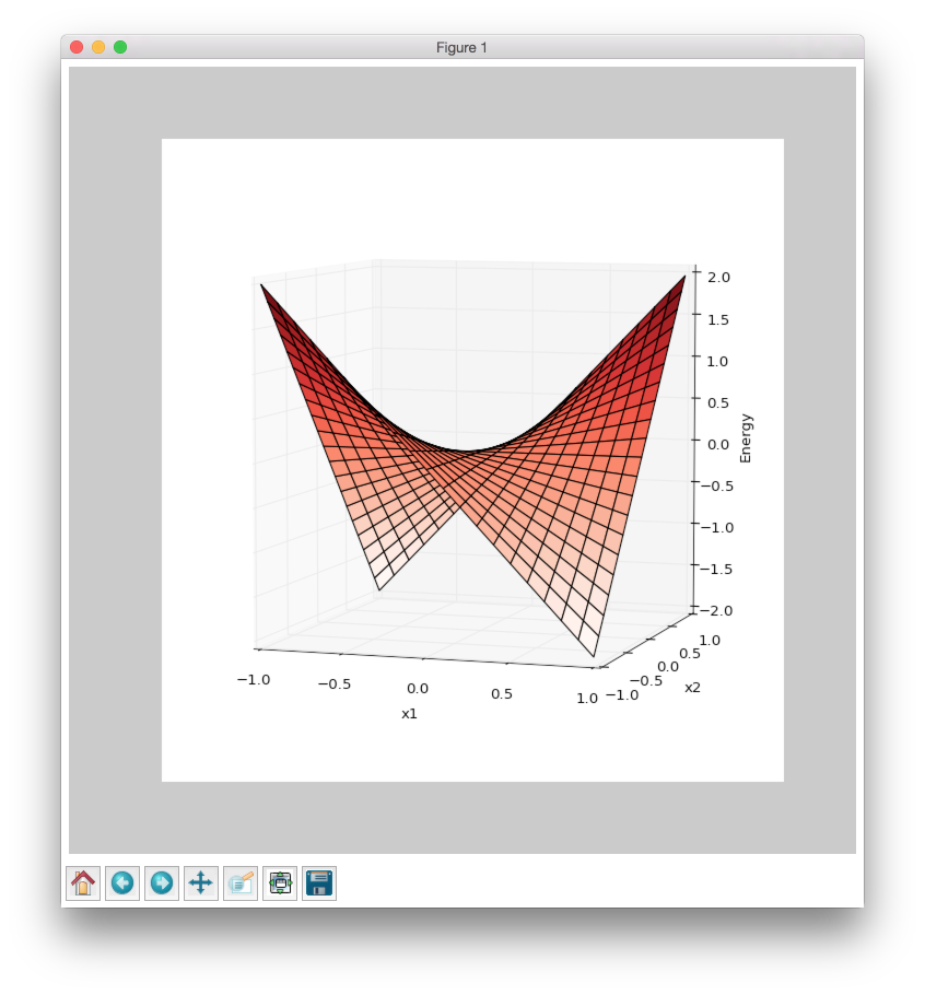
As you can see we have two minimum values at the same points as those patterns that are already stored inside the network. But between these two patterns function creates a saddle point somewhere at the point with coordinates \((0, 0)\). In this case we can’t stick to the points \((0, 0)\). But in situation with more dimensions this saddle points can be at the level of available values and they could be hallucination. Unfortunately, we are very limited in terms of numbers of dimensions we could plot, but the problem is still the same.
Full source code for this plot you can find on github
Example
Now we are ready for a more practical example. Let’s define a few images that we are going to teach the network.
>>> import numpy as np
>>> from neupy import algorithms
>>>
>>> def draw_bin_image(image_matrix):
...     for row in image_matrix.tolist():
...         print('| ' + ' '.join(' *'[val] for val in row))
...
>>> zero = np.matrix([
...     0, 1, 1, 1, 0,
...     1, 0, 0, 0, 1,
...     1, 0, 0, 0, 1,
...     1, 0, 0, 0, 1,
...     1, 0, 0, 0, 1,
...     0, 1, 1, 1, 0
... ])
>>>
>>> one = np.matrix([
...     0, 1, 1, 0, 0,
...     0, 0, 1, 0, 0,
...     0, 0, 1, 0, 0,
...     0, 0, 1, 0, 0,
...     0, 0, 1, 0, 0,
...     0, 0, 1, 0, 0
... ])
>>>
>>> two = np.matrix([
...     1, 1, 1, 0, 0,
...     0, 0, 0, 1, 0,
...     0, 0, 0, 1, 0,
...     0, 1, 1, 0, 0,
...     1, 0, 0, 0, 0,
...     1, 1, 1, 1, 1,
... ])
>>>
>>> draw_bin_image(zero.reshape((6, 5)))
|   * * *
| *       *
| *       *
| *       *
| *       *
|   * * *
We have 3 images, so now we can train network with these patterns.
>>> data = np.concatenate([zero, one, two], axis=0)
>>>
>>> dhnet = algorithms.DiscreteHopfieldNetwork(mode='sync')
>>> dhnet.train(data)
That’s all. Now to make sure that network has memorized patterns right we can define the broken patterns and check how the network will recover them.
>>> half_zero = np.matrix([
...     0, 1, 1, 1, 0,
...     1, 0, 0, 0, 1,
...     1, 0, 0, 0, 1,
...     0, 0, 0, 0, 0,
...     0, 0, 0, 0, 0,
...     0, 0, 0, 0, 0,
... ])
>>> draw_bin_image(half_zero.reshape((6, 5)))
|   * * *
| *       *
| *       *
|
|
|
>>>
>>> half_two = np.matrix([
...     0, 0, 0, 0, 0,
...     0, 0, 0, 0, 0,
...     0, 0, 0, 0, 0,
...     0, 1, 1, 0, 0,
...     1, 0, 0, 0, 0,
...     1, 1, 1, 1, 1,
... ])
>>> draw_bin_image(half_two.reshape((6, 5)))
|
|
|
|   * *
| *
| * * * * *
Now we can reconstruct pattern from the memory.
>>> result = dhnet.predict(half_zero)
>>> draw_bin_image(result.reshape((6, 5)))
|   * * *
| *       *
| *       *
| *       *
| *       *
|   * * *
>>>
>>> result = dhnet.predict(half_two)
>>> draw_bin_image(result.reshape((6, 5)))
| * * *
|       *
|       *
|   * *
| *
| * * * * *
Cool! Network catches the pattern right.
But not always we will get the correct answer. Let’s define another broken pattern and check network output.
>>> half_two = np.matrix([
...     1, 1, 1, 0, 0,
...     0, 0, 0, 1, 0,
...     0, 0, 0, 1, 0,
...     0, 0, 0, 0, 0,
...     0, 0, 0, 0, 0,
...     0, 0, 0, 0, 0,
... ])
>>>
>>> result = dhnet.predict(half_two)
>>> draw_bin_image(result.reshape((6, 5)))
|   * *
|     *
|     *
|   * *
| *   *
| * * * * *
We hasn’t clearly taught the network to deal with such pattern. But if we look closer, it looks like mixed pattern of numbers 1 and 2.
This problem we can solve using the asynchronous network approach. We don’t necessary need to create a new network, we can just simply switch its mode.
>>> from neupy import utils
>>> utils.reproducible()
>>>
>>> dhnet.mode = 'async'
>>> dhnet.n_times = 400
>>>
>>> result = dhnet.predict(half_two)
>>> draw_bin_image(result.reshape((6, 5)))
|   * *
|     *
|     *
|     *
|     *
|     *
>>> result = dhnet.predict(half_two)
>>> draw_bin_image(result.reshape((6, 5)))
| * * *
|       *
|       *
|   * *
| *
| * * * *
Our broken pattern is really close to the minimum of 1 and 2 patterns. Randomization helps us choose direction but it’s not necessary the right one, especially when the broken pattern is close to 1 and 2 at the same time.
Check last output with number two again. Is that a really valid pattern for number 2? Final symbol in output is wrong. We are not able to recover patter 2 from this network, because input vector is always much closer to the minimum that looks very similar to pattern 2.
In plot below you can see first 200 iterations of the recovery procedure. Energy value was decreasing after each iteration until it reached the local minimum where pattern is equal to 2.
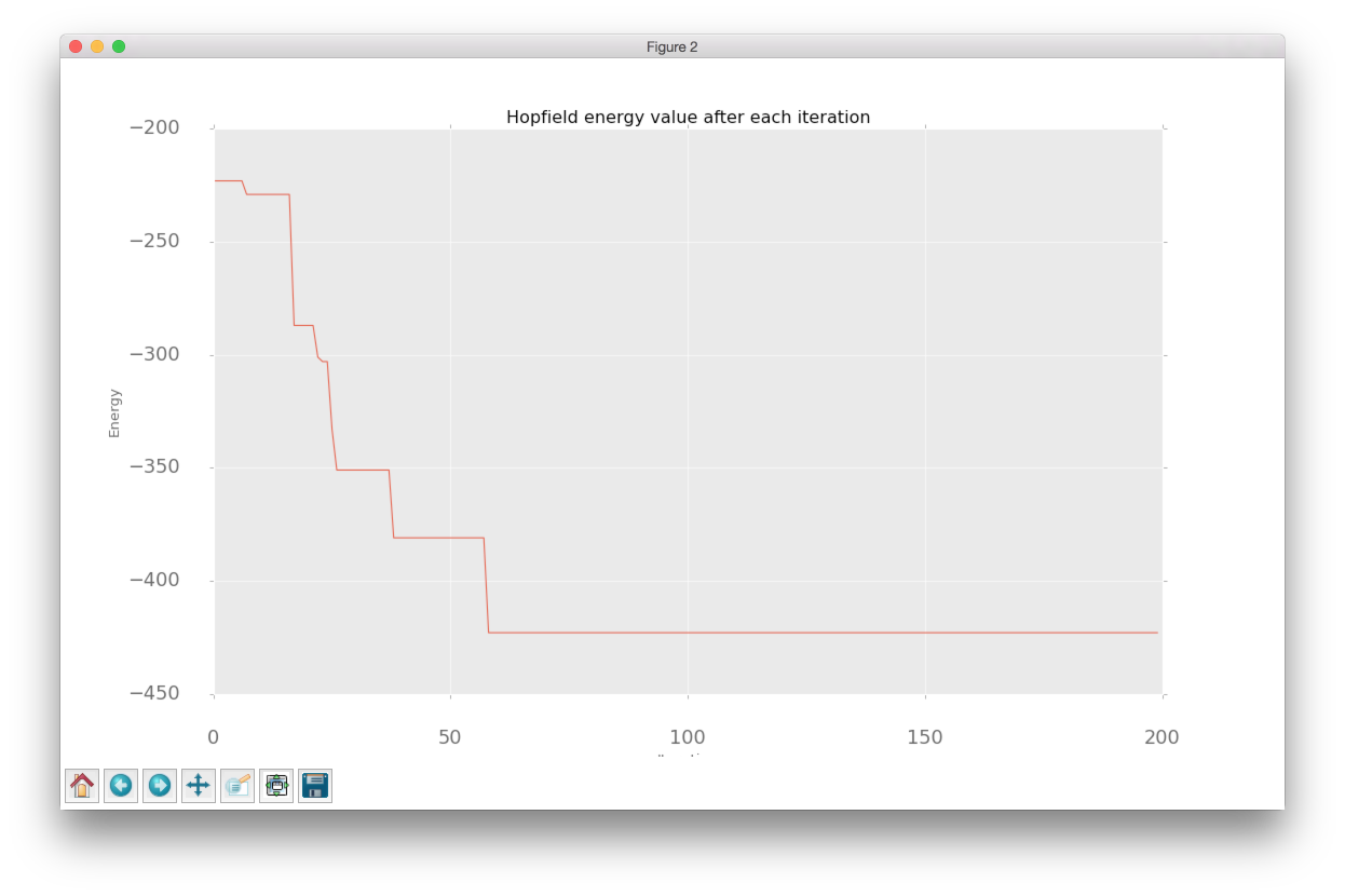
And finally we can look closer to the network memory using Hinton diagram.
>>> from neupy import plots
>>> import matplotlib.pyplot as plt
>>>
>>> plt.figure(figsize=(14, 12))
>>> plt.title("Hinton diagram")
>>> plots.hinton(dhnet.weight)
>>> plt.show()
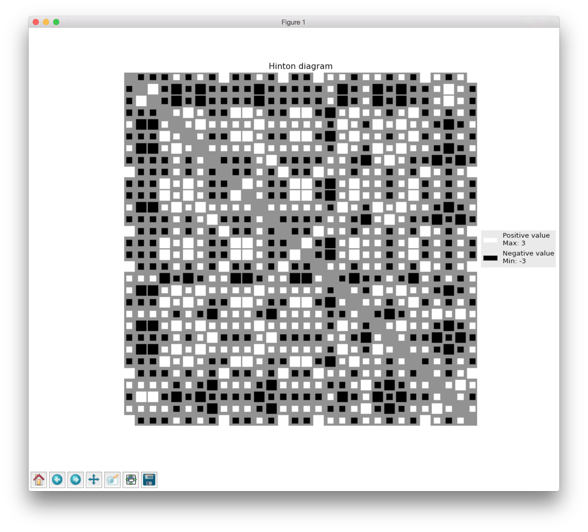
This graph above shows the network weight matrix and all information stored inside of it. Hinton diagram is a very simple technique for the weight visualization in neural networks. Each value encoded in square where its size is an absolute value from the weight matrix and color shows the sign of this value. White is a positive and black is a negative. Usually Hinton diagram helps identify some patterns in the weight matrix.
Let’s go back to the graph. What can you say about the network just by looking at this picture? First of all you can see that there is no squares on the diagonal. That is because they are equal to zero. The second important thing you can notice is that the plot is symmetrical. But that is not all that you can withdraw from the graph. Can you see different patterns? You can find rows or columns with exactly the same values, like the second and third columns. Fifth column is also the same but its sign is reversed. Now look closer to the antidiagonal. What can you say about it? If you are thinking that all squares are white - you are right. But why is that true? Is there always the same patterns for each memory matrix? No, it is a special property of patterns that we stored inside of it. If you draw a horizontal line in the middle of each image and look at it you will see that values are opposite symmetric. For instance, \(x_1\) opposite symmetric to \(x_{30}\), \(x_2\) to \(x_{29}\), \(x_3\) to \(x_{28}\) and so on. Zero pattern is a perfect example where each value have exactly the same opposite symmetric pair. One is almost perfect except one value on the \(x_2\) position. Two is not clearly opposite symmetric. But if you check each value you will find that more than half of values are symmetrical. Combination of those patterns gives us a diagonal with all positive values. If we have all perfectly opposite symmetric patterns then squares on the antidiagonal will have the same length, but in this case pattern for number 2 gives a little bit of noise and squares have different sizes.
Properties that we’ve reviewed so far are just the most interesting and maybe other patterns you can encounter on your own.
More reading
In addition you can read another article about a ‘Password recovery’ from the memory using the Discrete Hopfield Network.
References
| [1] | R. Rojas. Neural Networks. In Associative Networks. pp. 311 - 336, 1996. |
| [2] | Math4IQB. (2013, November 17). Hopfield Networks. Retrieved from https://www.youtube.com/watch?v=gfPUWwBkXZY |
| [3] | R. Callan. The Essence of Neural Networks. In Pattern Association. pp. 84 - 98, 1999. |
Predict prices for houses in the area of Boston
Boston house prices is a classical example of the regression problem. This article shows how to make a simple data processing and train neural network for house price forecasting.
Dataset can be downloaded from many different resources. In order to simplify this process we will use scikit-learn library. It will download and extract and the data for us.
from sklearn import datasets

dataset = datasets.load_boston()
data, target = dataset.data, dataset.target
We can print few first rows from the dataset just to make sure that
| CRIM | ZN | INDUS | CHAS | NOX | RM | AGE | DIS | RAD |
|---|---|---|---|---|---|---|---|---|
| 0.00632 | 18 | 2.31 | 0 | 0.538 | 6.575 | 65.2 | 4.0900 | 1 |
| 0.02731 | 0 | 7.07 | 0 | 0.469 | 6.421 | 78.9 | 4.9671 | 2 |
| 0.02729 | 0 | 7.07 | 0 | 0.469 | 7.185 | 61.1 | 4.9671 | 2 |
| 0.03237 | 0 | 2.18 | 0 | 0.458 | 6.998 | 45.8 | 6.0622 | 3 |
| 0.06905 | 0 | 2.18 | 0 | 0.458 | 7.147 | 54.2 | 6.0622 | 3 |
| TAX | PTRATIO | B | LSTAT | MEDV |
|---|---|---|---|---|
| 296 | 15.3 | 396.90 | 4.98 | 24.0 |
| 242 | 17.8 | 396.90 | 9.14 | 21.6 |
| 242 | 17.8 | 392.83 | 4.03 | 34.7 |
| 222 | 18.7 | 394.63 | 2.94 | 33.4 |
| 222 | 18.7 | 396.90 | 5.33 | 36.2 |
Data contains 14 columns. The last column MEDV is a median value of owner-occupied homes in $1000’s. The goal is to predict this value. Other columns we can use for neural network training.
It’s quite hard to understand data just from the column names. Scikit-learn also provides description.
print(dataset.DESCR)
- CRIM - per capita crime rate by town
- ZN - proportion of residential land zoned for lots over 25,000 sq.ft.
- INDUS - proportion of non-retail business acres per town
- CHAS - Charles River dummy variable (= 1 if tract bounds river; 0 otherwise)
- NOX - nitric oxides concentration (parts per 10 million)
- RM - average number of rooms per dwelling
- AGE - proportion of owner-occupied units built prior to 1940
- DIS - weighted distances to five Boston employment centres
- RAD - index of accessibility to radial highways
- TAX - full-value property-tax rate per $10,000
- PTRATIO - pupil-teacher ratio by town
- B - 1000(Bk - 0.63)^2 where Bk is the proportion of blacks by town
- LSTAT - % lower status of the population
There are 13 continuous attributes (including “class” attribute “MEDV”) and 1 binary-valued attribute. There are no columns that have multiple categories, which simplifies initial data processing..
From the table above you can notice that every column has values in different scales. It might slow down or completely break networks convergence. In order to fix this issue, we should normalize values in every column. One of the simplest way to do it is to map every value into range between 0 and 1, where maximum value in every column will be equal to 1 and the smallest one - to 0.
from sklearn import preprocessing

data_scaler = preprocessing.MinMaxScaler()
target_scaler = preprocessing.MinMaxScaler()

data = data_scaler.fit_transform(data)
target = target_scaler.fit_transform(target.reshape(-1, 1))
After transformation data looks like this.
| CRIM | ZN | INDUS | CHAS | NOX | ... |
|---|---|---|---|---|---|
| 0.000000 | 0.18 | 0.067815 | 0 | 0.314815 | ... |
| 0.000236 | 0.00 | 0.242302 | 0 | 0.172840 | ... |
| 0.000236 | 0.00 | 0.242302 | 0 | 0.172840 | ... |
| 0.000293 | 0.00 | 0.063050 | 0 | 0.150206 | ... |
| 0.000705 | 0.00 | 0.063050 | 0 | 0.150206 | ... |
Neural networks are prune to overfitting and we always need to have validation dataset that we will use to assess networks performance after the training.
from sklearn.model_selection import train_test_split
from neupy import utils

# Make sure that split between train and
# validation datasets will be reproducible
utils.reproducible()

x_train, x_test, y_train, y_test = train_test_split(
    # 85% of the data we will use for training
    # and the other 15% will be used for validation
    data, target, test_size=0.15
)
Since we have all the data the last thing that we need is a neural network. We can design simple network with only one hidden layer.
from neupy.layers import *

# Number of features that we want
# to use during the training
n_inputs = 13

# Number of outputs in the network. For the house price
# forecasting we want to predict single value per every
# input sample.
n_outputs = 1

network = join(
    # This layer doesn't do any computation. It just
    # defines how many inputs network should expect.
    Input(n_inputs),

    # Hidden layer. Number of neurons can be adjusted
    # in order to improve performance or deal with overfitting
    Sigmoid(50),

    # Sigmoid outputs values between 0 and 1 and all
    # the prices that we want to predict has been rescaled
    # to the same range.
    Sigmoid(n_outputs),
)
Now that we have the our network we can use one of the large training algorithms supported by neupy. Our datasets is quite small and network has small number of parameters. For cases like this we can take advantage of the more algorithms that can converge much faster. I’ll use Levenberg-Marquardt, but you can feel free to experiment with different algorithms.
from neupy import algorithms

optimizer = algorithms.LevenbergMarquardt(
    # First argument has to be neural network
    network,

    # With this option enabled network shows its configuration
    # before the training and its progress during the training
    verbose=True,

    # In order to avoid showing information about
    # network training progress after every epoch we can
    # do it less frequently, for example, every 5th epoch.
    show_epoch=5,
)
Output after initialization might look like this
Main information

[ALGORITHM] LevenbergMarquardt

[OPTION] loss = mse
[OPTION] mu = 0.01
[OPTION] mu_update_factor = 1.2
[OPTION] show_epoch = 5
[OPTION] shuffle_data = False
[OPTION] signals = None
[OPTION] target = Tensor("placeholder/target/sigmoid-10:0", shape=(?, 1), dtype=float32)
[OPTION] verbose = True

[TENSORFLOW] Initializing Tensorflow variables and functions.
[TENSORFLOW] Initialization finished successfully. It took 0.30 seconds
And finally, we can use our data in order to train the network. In addition, neupy allows to specify validation datasets. It won’t use it for training. Instead, at the end of every epoch it will use validation data to estimate network forecasting performance on the unseen data.
optimizer.train(x_train, y_train, x_test, y_test, epochs=30)
Output during the training might look like this
#1 : [224 ms] train: 0.046980, valid: 0.032002
#5 : [76 ms] train: 0.009437, valid: 0.013484
#10 : [75 ms] train: 0.007141, valid: 0.010253
#15 : [77 ms] train: 0.004664, valid: 0.008936
#20 : [75 ms] train: 0.003780, valid: 0.009333
#25 : [75 ms] train: 0.003117, valid: 0.008975
#30 : [77 ms] train: 0.002608, valid: 0.009507
It’s also useful to visualize network training progress using line plot. In the figure below you can see two lines. One line shows training error and the other one validation error.
optimizer.plot_errors()
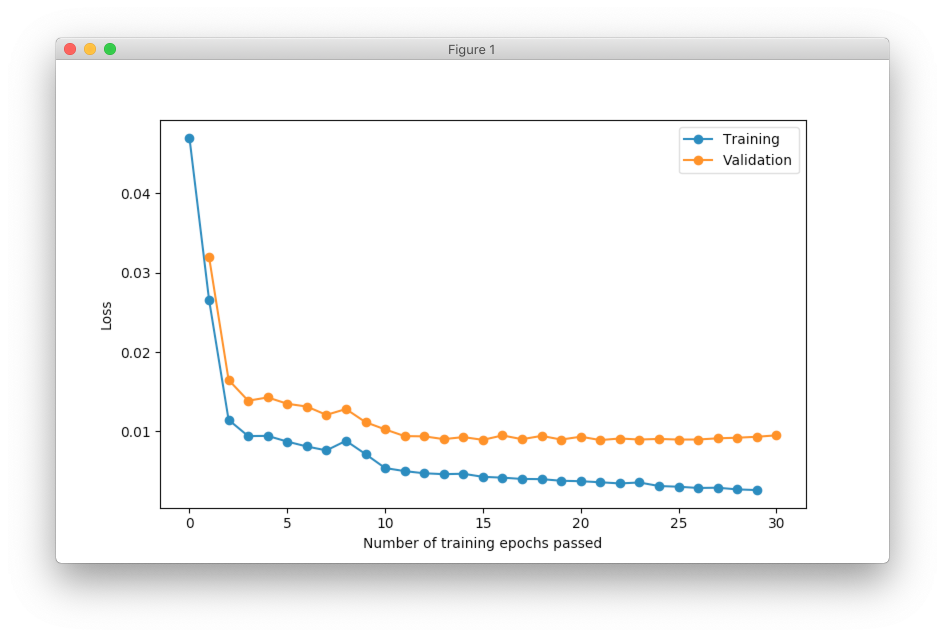
We typically want to see decrease for the validation error. The training error might be useful during debugging. For example, it might be used in order to see if network overfits.
During the training we used mean squared error as a loss function on the scaled prediction values. We can use different function in order to measure network’s forecasting performance. For example, we can use Root Means Squared Logarithmic Error (RMSLE) and compare prediction to the exact value that were scaled back to the original scale.
import numpy as np

def rmsle(expected, predicted):
    log_expected = np.log1p(expected + 1)
    log_predicted = np.log1p(predicted + 1)
    squared_log_error = np.square(log_expected - log_predicted)
    return np.sqrt(np.mean(squared_log_error))

y_predict = optimizer.predict(x_test).round(1)
error = rmsle(
    target_scaler.inverse_transform(y_test),
    target_scaler.inverse_transform(y_predict),
)
print(error)  # ~0.18
The final result is quite good for the first prototype.