Earthquakes in the Landscape of Neural Network
In this article, I want to direct your attention to the less known properties of one, quite famous, technique in the deep learning. I want to show you how beautiful and interesting could be a concept that typically left behind because of all more exciting ideas in this area.
Introduction
Artificial neural networks have been proven to be a very powerful tool for solving a wide variety of problems. Large number of researchers and engineers put their time and effort to develop the field, although there is still a lot to discover. And because of that, field evolves so quickly that large number of architectures and techniques that were popular just a few years ago, now is a part of the history. But not everything gets outdated and certain techniques prove to be useful to such an extent that it’s hard to imagine deep learning without them.
In this article, I want to direct your attention to the less known properties of one, quite famous, technique in the deep learning. I want to show you how beautiful and interesting could be a concept that typically left behind because of all more exciting ideas in this area.
What can you see?
Until now, I haven’t explained this mysterious “earthquake” phenomena and I would like to keep it like this for a little longer. I want to encourage you to focus on the properties of this phenomena and see whether you can recognize something that, most likely, is known to you.
As I mentioned earlier, certain clues could be revealed from the animation. In order to simplify things, we can focus our attention on a single frame and see what we can find.
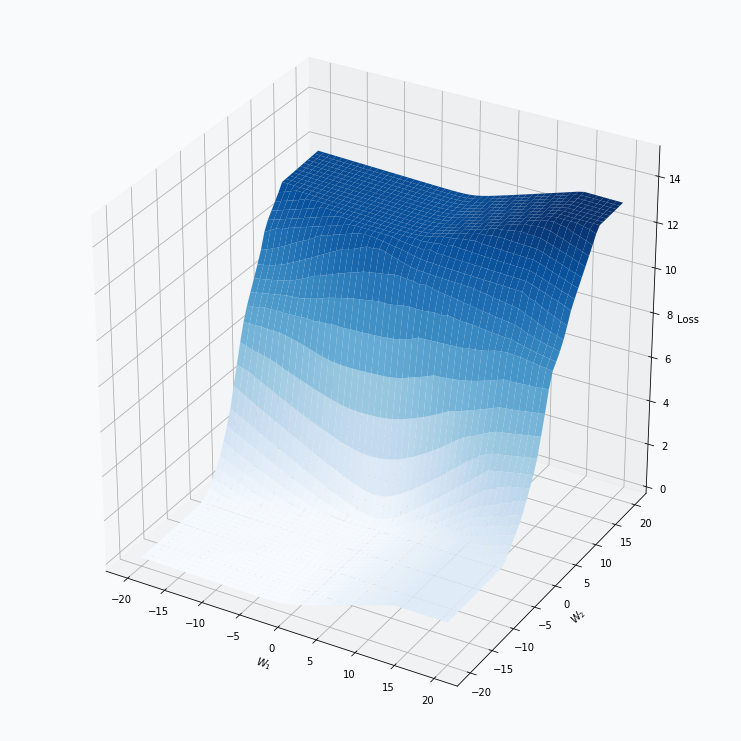
Some of you should be familiar with the graph like this. There we can see three axes, namely \(W_1\), \(W_2\) and Loss. Two of the axes specify different parameters/weights of the network, namely \(W_1\) and \(W_2\). The last axis shows a loss associated with each possible pair of parameters \(W_1\) and \(W_2\). That’s how neural network’s loss landscape looks like. Typically, during the training, we start with some fixed values \(W_1\), \(W_2\) and, with the help of an algorithm, like gradient descent, we navigate around landscape trying to find weights associated with lowest value on this surface. Assuming that this part is clear, one question still remains: Why does the loss landscape changes on the animation?
Let’s think what does this change represent. For each fixed pair of weights \(W_1\), \(W_2\) the loss value, associated with them, changes. And from this perspective it shouldn’t be that surprising, since we will never expect network to have exactly the same loss associated with a fixed set of weights. And at this point I would like to stop, since we’re getting pretty close to the answer.
I would encourage you to take a moment, think about what we’ve observed so far from the animation and guess what might produce this effect on the loss landscape. I suggest you to do it now, because next section contains an explanation of this phenomena.
Explanation
The animation shows how the neural network’s loss landscape looks like during the training with mini-batches. It’s quite common to think of a surface as a static landscape where we navigate during the training, trying to find weights that minimize desirable loss function. This statement might be considered as true only in case of the full-batch training, when all the available data samples are used at the same time during the training. But for most of the deep learning problems, that statement is false. During the training, we navigate in dynamically changing environment. For each training iteration, we take a set of input samples, propagate them thought the network and estimate gradient which we will use to adjust network’s weights.
It might be easier to visualize training using contour plots. The same 3D animation could be represented in the following way:
Animation above shows only the way the loss landscape changes when we use different mini-batches, but it doesn’t show us its effect on the training. We can extend this animation with gradient vectors.
Animation above alternates between two steps, namely training iteration and mini-batch changing. Training iteration shows static landscape and vector shows how the weights have changed after the update. Next training iteration requires different mini-batch and this changeover is visualized by the smooth transition between two landscapes. In reality, this change is not smooth, but animation helps us to notice the effect of that change. The bigger the difference between two losses the more noticeable will be transition between two landscapes.
After completing multiple training iterations, we can see that the overall path looks a bit noisy. During each iteration gradient point towards the direction that minimizes the loss but continuous changes in the loss landscape makes it quite difficult to find a stable direction. This problem could be minimized with algorithms that accumulate information about a gradient over time. If you want to learn more about that you can check this article.
Mathematical perspective
Unlike in mathematical optimization, in neural networks, we don’t know what function we want to optimize. It sounds a bit strange, but that’s true. Each mini-batch creates a different loss landscape and during each iteration we optimize different function. With random shuffling and reasonably large mini-batch size, it’s quite unlikely that we will see exactly the same loss landscape twice during the training. It sounds even a bit surreal, if you think about it. We move towards the minimum of the function which we most likely won’t see ever again and somehow optimization algorithm arrives at a solution that works incredibly well for a target task, e.g. image classification.
Most of the loss functions used in deep learning calculate loss independently per each input sample and the overall loss will be just an average of these losses. Notice, that this property helps us to obtain gradient very easily, since the gradient of the average is the average of the gradients per each individual addend.
where, N is the number of samples in a mini-batch, E is a total loss, \(e_i\) is a loss associated with i-th input sample.
We can think that during the training we randomly sample loss landscapes and use average loss landscape in order to estimate the gradient. For example, we can take 9 random input samples and create loss landscape per each individual sample. By averaging these landscapes, we can obtain new landscape.
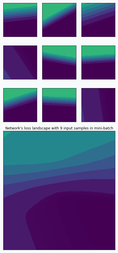
On the graph above, you can notice that 9 loss landscapes have linear contours and the averaged loss landscape doesn’t have this property. Each individual loss landscape has been obtained from a cross entropy loss function and simple logistic regression as a base network architecture. It could be easily shown that each individual loss is nearly piecewise linear function.
where \(x\) is an input vector, \(y \in \{0, 1\}\) is a target class and \(w\) is a vector with network’s parameters.
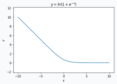
Obtained result could be separated into 2 parts. The first part is just a linear transformation of the input \(x\). The second part is a logarithm, but it behaves like a linear function when the absolute value of the \(x^T w\) is reasonably large.
Statistical perspective
We can also think about mini-batch training in terms of the loss landscape sampling. In statistics, random sampling helps us to derive properties of the entire population using summary statistics. For example, we might estimate expected value from the population by calculating average over a random sample. Obviously, the smaller sample we get, the less certain we’re about our estimation. And the same is true (or rather nearly true) for loss landscape sampling. This effect was demonstrated on the first animation:
I used mini-batch of size 10 for the graph on the left and size 100 for the graph on the right. We can see that “earthquake” effect is stronger for the left graph, where mini-batch size is smaller. Basically, estimation of the loss landscape, produced by small mini-batch, has quite large variance and it could be observed from the animation.
I want to make one disclaimer about sampling. It’s not quite the same as I’ve defined it for the statistical inference. Training dataset is already a sample from a population and each mini-batch is a sample from this sample. In addition to that, each mini-batch is not sampled independently. Typically, before each training epoch, we shuffle samples in our dataset and divide them into mini-batches. Propagation of the first mini-batch has an impact on the data distribution in the next mini-batch. For example, imagine simple problem where we try to classify 0 and 1 digits (binary classification on binary digits). In addition, we can imagine that in our training dataset, there are as many 0s as 1s. Imagine that in the first mini-batch we have more 1s than 0s. It means that in the rest of the training dataset we have more 0s than 1s and for the next mini-batch, we’re more likely to get more 0s than 1s, since probability was skewed by the first mini-batch. Whether it’s good, bad or shouldn’t matter, might be a separate topic for a different article, but the fact is that this sampling is not purely random.
Final words
In my opinion, term earthquake fits very naturally into a general intuition about neural network training. If you think about loss landscape as an area with mountains and valleys then earthquake represents shakes and displacement of that land. Magnitude of that earthquake could be measured with a size of the mini-batch. And navigation in this environment could be compared to the training with momentum.
Code
All the code, that has been used to generate graphs and animations for this article, could be found on Github.