Visualizations
Training progress
Optimizers that used for training neural networks with constructible architectures have separate method that called plot_errors. This method provides basic information about training.
from neupy import algorithms
from neupy.layers import *

network = Input(10) >> Sigmoid(20) >> Sigmoid(1)
optimizer = algorithms.Adadelta(network, batch_size=10)

x_train, x_test, y_train, y_test = load_data()
optimizer.train(x_train, y_train, x_test, y_test, epochs=100)

optimizer.plot_errors()
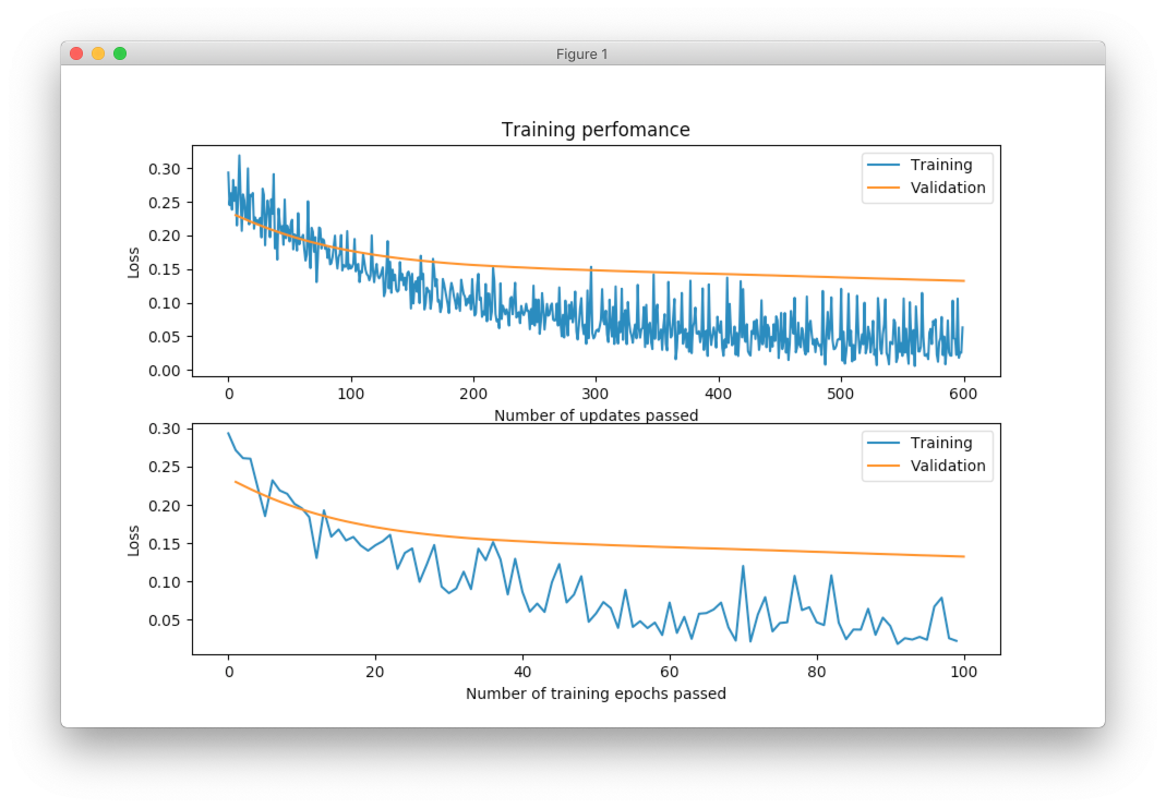
You can notice how noise is that training curve compare to the validation curve. The reason for it is because we used batch size equal to 10 that loss estimation is quite noisy for such a small sample, whether whole validation set was used for the loss estimation and therefor loss curve is much smoother.
When only small number of epochs was specified for the training it’s easy to see one mismatch between curves, it’s is if one of the shifted be one unit.
network = Input(10) >> Sigmoid(20) >> Sigmoid(1)
optimizer = algorithms.Adadelta(network, batch_size=None)

optimizer.train(x_train, y_train, x_test, y_test, epochs=10)
optimizer.plot_errors()
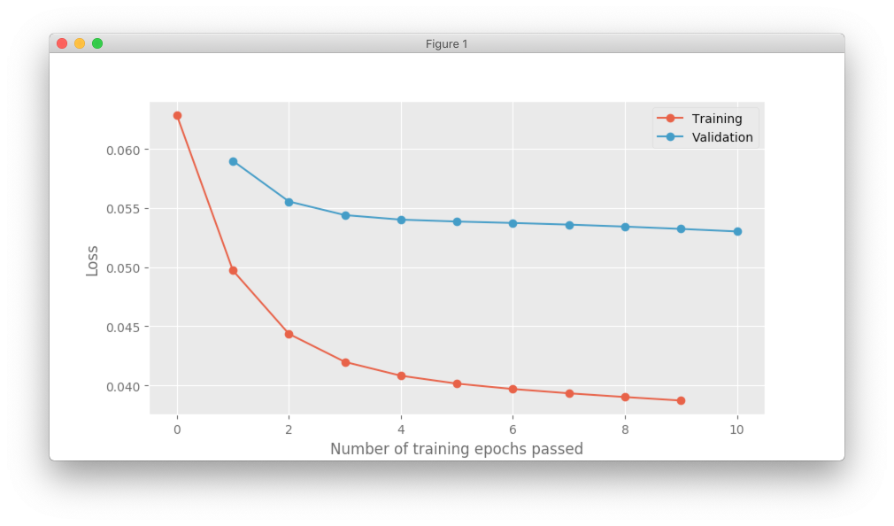
First of all, notice that now we have only one plot. It’s because we have batch_size=None. When during every epoch we propagate single batch there is no difference between number of updates and number of epochs. Second, notice that that training curve starts at position 0 and validation curve at position 1. The reason for it is quite simple. When we pass first batch of the training data through the network, we calculate the loss. This loss has been calculated before we updated weights and therefor no updates has been made yet. After that we use our loss to estimate gradients and apply updates to the weights. When updates were applied we can use our validation data in order to estimate validation loss, but this time we’ve already done one update for the weights. It will be wrong to put training and validation loss one on top of the other, since they’ve calculated losses in different states of the neural network parameters. Next epoch, training data will calculate losses using weights that has been updated one time and now we have data point that’s relevant to the validation loss calculated in the previous epoch.
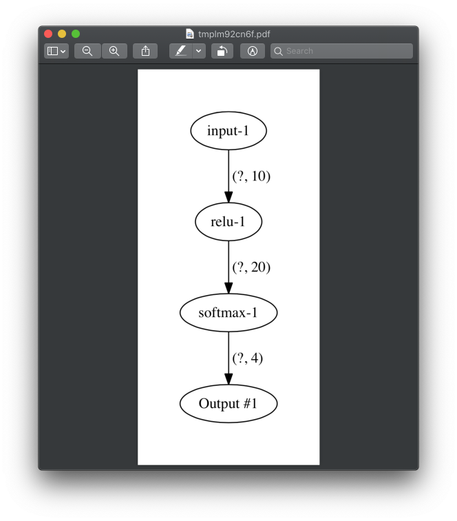
Network structure
Relations between layers in the network can be visualized using the show method that can be accessed from any network.
from neupy.layers import *
network = Input(10) >> Relu(20) >> Softmax(4)
network.show()
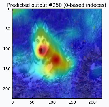
Saliency Map
Learn more details about the saliency_map function from the documentation.
from neupy import plots

vgg19 = ...  # define pretrained VGG19 network
dog_image = ...  # load image of dog

# apply preprocessing step to dog image
processed_dog_image = process(dog_image)

plt.imshow(dog_image)
plots.saliency_map(vgg19, processed_dog_image, alpha=0.6, sigma=10)
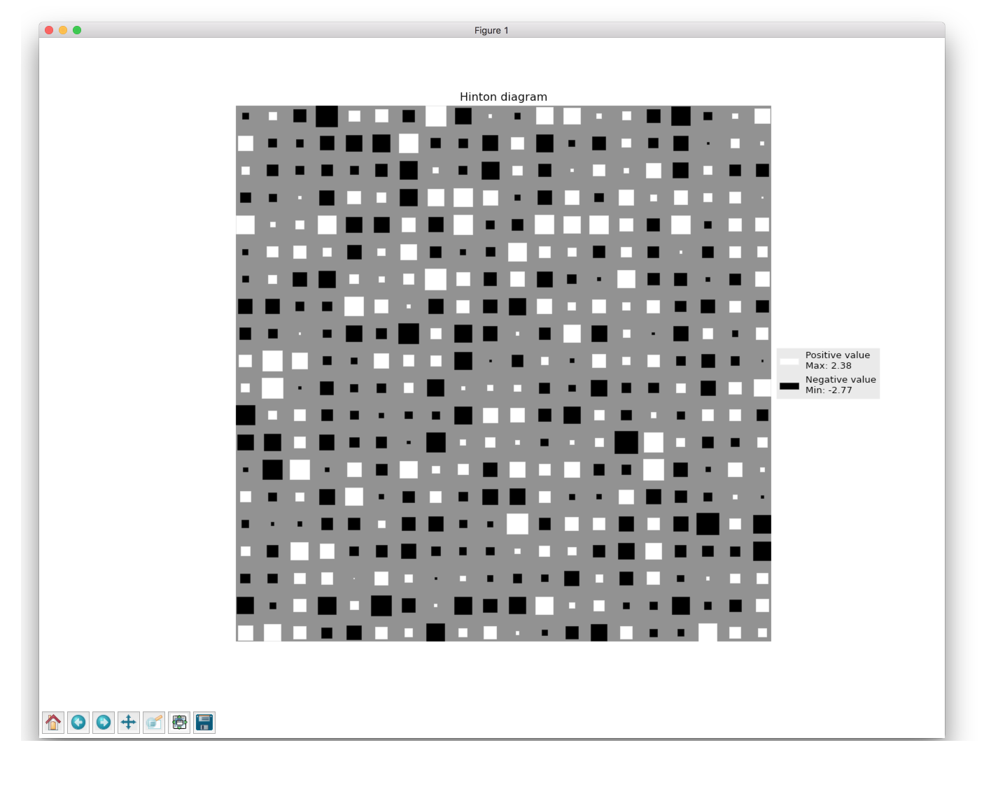
Hinton diagram
More information about the Hinton diagram you can find in documentation.
import numpy as np
import matplotlib.pyplot as plt
from neupy import plots

weight = np.random.randn(20, 20)

plt.style.use('ggplot')
plt.figure(figsize=(16, 12))
plt.title("Hinton diagram")
plots.hinton(weight)
plt.show()